Large dynamic factor models, forecasting, and nowcasting(Open on Google Colab | View / download notebook | Report a problem)
Table of Contents
Large dynamic factor models, forecasting, and nowcasting
Dynamic factor models postulate that a small number of unobserved “factors” can be used to explain a substantial portion of the variation and dynamics in a larger number of observed variables. A “large” model typically incorporates hundreds of observed variables, and estimating of the dynamic factors can act as a dimension-reduction technique. In addition to producing estimates of the unobserved factors, dynamic factor models have many uses in forecasting and macroeconomic monitoring. One popular application for these models is “nowcasting”, in which higher-frequency data is used to produce “nowcasts” of series that are only published at a lower frequency.
Table of Contents
This notebook describes working with these models in Statsmodels, using the DynamicFactorMQ class:
- Brief overview
- Dataset
- Specifying a mixed-frequency dynamic factor model with several blocks of factors
- Model fitting / parameter estimation
- Estimated factors
- Forecasting observed variables
- Nowcasting GDP, real-time forecast updates, and a decomposition of the “news” from updated datasets
- References
Note: this notebook is compatible with Statsmodels v0.12 and later. It will not work with Statsmodels v0.11 and earlier.
%matplotlib inline

import types
import numpy as np
import pandas as pd
import statsmodels.api as sm

import matplotlib.pyplot as plt
import seaborn as sns
Brief overview
The dynamic factor model considered in this notebook can be found in the DynamicFactorMQ class, which is a part of the time series analysis component (and in particular the state space models subcomponent) of Statsmodels. It can be accessed as follows:
import statsmodels.api as sm
model = sm.tsa.DynamicFactorMQ(...)
Data
In this notebook, we’ll use 127 monthly variables and 1 quarterly variable (GDP) from the FRED-MD / FRED-QD dataset (McCracken and Ng, 2016).
Statistical model:
The statistical model and the EM-algorithm used for parameter estimation are described in:
- Bańbura and Modugno (2014), “Maximum likelihood estimation of factor models on datasets with arbitrary pattern of missing data.” (Working paper, Published), and
- Bańbura et al. (2011), “Nowcasting” (Working paper, Handbook chapter)
As in these papers, the basic specification starts from the typical “static form” of the dynamic factor model:
\[\begin{aligned} y_t & = \Lambda f_t + \epsilon_t \\ f_t & = A_1 f_{t-1} + \dots + A_p f_{t-p} + u_t \end{aligned}\]The DynamicFactorMQ class allows for the generalizations of the model described in the references above, including:
- Limiting blocks of factors to only load on certain observed variables
- Monthly and quarterly mixed-frequency data, along the lines described by Mariano and Murasawa (2010)
- Allowing autocorrelation (via AR(1) specifications) in the idiosyncratic disturbances $\epsilon_t$
- Missing entries in the observed variables $y_t$
Parameter estimation
When there are a large number of observed variables $y_t$, there can be hundreds or even thousands of parameters to estimate. In this situation, it can be extremely difficult for the typical quasi-Newton optimization methods (which are employed in many of the Statsmodels time series models) to find the parameters that maximize the likelihood function. Since this model is designed to support a large panel of observed variables, the EM-algorithm is instead used, since it can be more robust (see the above references for details).
In particular, the model above is in state space form, and so the state space library in Statsmodels can be used to apply the Kalman filter and smoother routines that are required for estimation.
Forecasting and interpolation
Because the model is in state space form, once the parameters are estimated, it is straightforward to produce forecasts of any of the observed variables $y_t$.
In addition, for any missing entries in the observed variables $y_t$, it is also straightforward to produce estimates of those entries based on the factors extracted from the entire observed dataset (“smoothed” factor estimates). In a monthly/quarterly mixed frequency model, this can be used to interpolate monthly values for quarterly variables.
Nowcasting, updating forecasts, and computing the “news”
By including both monthly and quarterly variables, this model can be used to produce “nowcasts” of a quarterly variable before it is released, based on the monthly data for that quarter. For example, the advance estimate for the first quarter GDP is typically released in April, but this model could produce an estimate in March that was based on data through February.
Many forecasting and nowcasting exercises are updated frequently, in “real time”, and it is therefore important that one can easily add new datapoints as they come in. As these new datapoints provide new information, the model’s forecast / nowcast will change with new data, and it is also important that one can easily decompose these changes into contributions from each updated series to changes in the forecast. Both of these steps are supported by all state space models in Statsmodels – including the DynamicFactorMQ model – as we show below.
Other resources
The New York Fed Staff Nowcast is an application of this same dynamic factor model and (EM algorithm) estimation method. Although they use a different dataset, and update their results weekly, their underlying framework is the same as that used in this notebook.
For more details on the New York Fed Staff Nowcast model and results, see Bok et al. (2018).
Dataset
In this notebook, we estimate a dynamic factor model on a large panel of economic data released at a monthly frequency, along with GDP, which is only released at a quarterly frequency. The monthly datasets that we’ll be using come from FRED-MD database (McCracken and Ng, 2016), and we will take real GDP from the companion FRED-QD database.
Data vintage
The FRED-MD dataset was launched in January 2015, and vintages are available for each month since then. The FRED-QD dataset was fully launched in May 2018, and monthly vintages are available for each month since then. Our baseline exercise will use the February 2020 dataset (which includes data through reference month January 2020), and then we will examine how updated incoming data in the months of March - June influenced the model’s forecast of real GDP growth in 2020Q2.
Data transformations
The assumptions of the dynamic factor model in this notebook require that the factors and observed variables are stationary. However, this dataset contains raw economic series that clearly violate that assumptions – for example, many of them show distinct trends. As is typical in these exercises, we therefore transform the variables to induce stationarity. In particular, the FRED-MD and FRED-QD datasets include suggested transformations (coded 1-7, which typically apply differences or percentage change transformations) which we apply.
The exact details are in the transform function, below:
def transform(column, transforms):
    transformation = transforms[column.name]
    # For quarterly data like GDP, we will compute
    # annualized percent changes
    mult = 4 if column.index.freqstr[0] == 'Q' else 1

    # 1 => No transformation
    if transformation == 1:
        pass
    # 2 => First difference
    elif transformation == 2:
        column = column.diff()
    # 3 => Second difference
    elif transformation == 3:
        column = column.diff().diff()
    # 4 => Log
    elif transformation == 4:
        column = np.log(column)
    # 5 => Log first difference, multiplied by 100
    #      (i.e. approximate percent change)
    #      with optional multiplier for annualization
    elif transformation == 5:
        column = np.log(column).diff() * 100 * mult
    # 6 => Log second difference, multiplied by 100
    #      with optional multiplier for annualization
    elif transformation == 6:
        column = np.log(column).diff().diff() * 100 * mult
    # 7 => Exact percent change, multiplied by 100
    #      with optional annualization
    elif transformation == 7:
        column = ((column / column.shift(1))**mult - 1.0) * 100

    return column
Outliers
Following McCracken and Ng (2016), we remove outliers (setting their value to missing), defined as observations that are more than 10 times the interquartile range from the series mean.
However, in this exercise we are interested in “nowcasting” real GDP growth for 2020Q2, which was greatly affected by economic shutdowns stemming from the COVID-19 pandemic. During the first half of 2020, there are a number of series which include extreme observations, many of which would be excluded by this outlier test. Because these observations are likely to be informative about real GDP in 2020Q2, we only remove outliers for the period 1959-01 through 2019-12.
The details of outlier removal are in the remove_outliers function, below:
def remove_outliers(dta):
    # Compute the mean and interquartile range
    mean = dta.mean()
    iqr = dta.quantile([0.25, 0.75]).diff().T.iloc[:, 1]

    # Replace entries that are more than 10 times the IQR
    # away from the mean with NaN (denotes a missing entry)
    mask = np.abs(dta) > mean + 10 * iqr
    treated = dta.copy()
    treated[mask] = np.nan

    return treated
Loading the data
The load_fredmd_data function, below, performs the following actions, once for the FRED-MD dataset and once for the FRED-QD dataset:
- Based on the
vintageargument, it downloads a particular vintage of these datasets from the base URL https://s3.amazonaws.com/files.fred.stlouisfed.org/fred-md into theorig_[m|q]variable. - Extracts the column describing which transformation to apply into the
transform_[m|q](and, for the quarterly dataset, also extracts the column describing which factor an earlier paper assigned each variable to). - Extracts the observation date (from the “sasdate” column) and uses it as the index of the dataset.
- Applies the transformations from step (2).
- Removes outliers for the period 1959-01 through 2019-12.
Finally, these are collected into an easy-to-use object (the SimpleNamespace object) and returned.
def load_fredmd_data(vintage):
    base_url = 'https://s3.amazonaws.com/files.fred.stlouisfed.org/fred-md'

    # - FRED-MD --------------------------------------------------------------
    # 1. Download data
    orig_m = (pd.read_csv(f'{base_url}/monthly/{vintage}.csv')
                .dropna(how='all'))

    # 2. Extract transformation information
    transform_m = orig_m.iloc[0, 1:]
    orig_m = orig_m.iloc[1:]

    # 3. Extract the date as an index
    orig_m.index = pd.PeriodIndex(orig_m.sasdate.tolist(), freq='M')
    orig_m.drop('sasdate', axis=1, inplace=True)

    # 4. Apply the transformations
    dta_m = orig_m.apply(transform, axis=0,
                         transforms=transform_m)

    # 5. Remove outliers (but not in 2020)
    dta_m.loc[:'2019-12'] = remove_outliers(dta_m.loc[:'2019-12'])

    # - FRED-QD --------------------------------------------------------------
    # 1. Download data
    orig_q = (pd.read_csv(f'{base_url}/quarterly/{vintage}.csv')
                .dropna(how='all'))

    # 2. Extract factors and transformation information
    factors_q = orig_q.iloc[0, 1:]
    transform_q = orig_q.iloc[1, 1:]
    orig_q = orig_q.iloc[2:]

    # 3. Extract the date as an index
    orig_q.index = pd.PeriodIndex(orig_q.sasdate.tolist(), freq='Q')
    orig_q.drop('sasdate', axis=1, inplace=True)

    # 4. Apply the transformations
    dta_q = orig_q.apply(transform, axis=0,
                          transforms=transform_q)

    # 5. Remove outliers (but not in 2020)
    dta_q.loc[:'2019Q4'] = remove_outliers(dta_q.loc[:'2019Q4'])

    # - Output datasets ------------------------------------------------------
    return types.SimpleNamespace(
        orig_m=orig_m, orig_q=orig_q,
        dta_m=dta_m, transform_m=transform_m,
        dta_q=dta_q, transform_q=transform_q, factors_q=factors_q)
We will call this load_fredmd_data function for each vintage from February 2020 through June 2020.
# Load the vintages of data from FRED
dta = {date: load_fredmd_data(date)
       for date in ['2020-02', '2020-03', '2020-04', '2020-05', '2020-06']}
# Print some information about the base dataset
n, k = dta['2020-02'].dta_m.shape
start = dta['2020-02'].dta_m.index[0]
end = dta['2020-02'].dta_m.index[-1]

print(f'For vintage 2020-02, there are {k} series and {n} observations,'
      f' over the period {start} to {end}.')
For vintage 2020-02, there are 128 series and 733 observations, over the period 1959-01 to 2020-01.
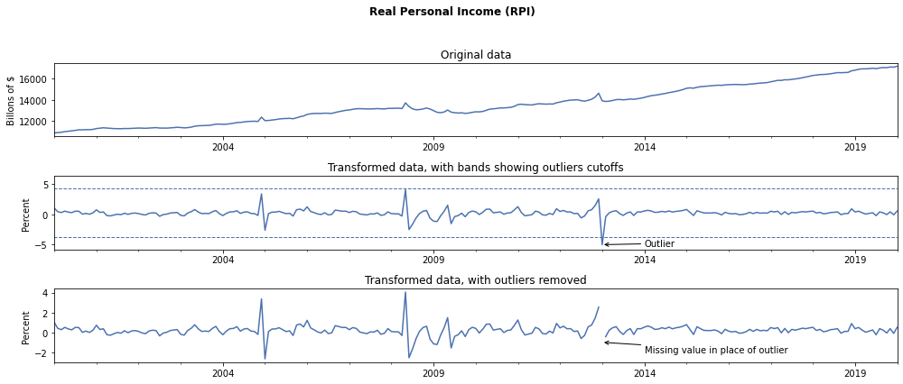
To see how the transformation and outlier removal works, here we plot three graphs of the RPI variable (“Real Personal Income”) over the period 2000-01 - 2020-01:
- The original dataset (which is in Billions of Chained 2012 Dollars)
- The transformed data (RPI had a transformation code of “5”, corresponding to log first difference)
- The transformed data, with outliers removed
Notice that the large negative growth rate in January 2013 was deemed to be an outlier and so was replaced with a missing value (a NaN value).
The BEA release at the time noted that this was related to “the effect of special factors, which boosted employee contributions for government social insurance in January [2013] and which had boosted wages and salaries and personal dividends in December [2012].”.
with sns.color_palette('deep'):
    fig, axes = plt.subplots(3, figsize=(14, 6))

    # Plot the raw data from the February 2020 vintage, for:
    #
    vintage = '2020-02'
    variable = 'RPI'
    start = '2000-01'
    end = '2020-01'

    # 1. Plot the original dataset, for 2000-01 through 2020-01
    dta[vintage].orig_m.loc[start:end, variable].plot(ax=axes[0])
    axes[0].set(title='Original data', xlim=('2000','2020'), ylabel='Billons of $')

    # 2. Plot the transformed data, still including outliers
    # (we only stored the transformation with outliers removed, so
    # here we'll manually perform the transformation)
    transformed = transform(dta[vintage].orig_m[variable],
                            dta[vintage].transform_m)
    transformed.loc[start:end].plot(ax=axes[1])
    mean = transformed.mean()
    iqr = transformed.quantile([0.25, 0.75]).diff().iloc[1]
    axes[1].hlines([mean - 10 * iqr, mean + 10 * iqr],
                   transformed.index[0], transformed.index[-1],
                   linestyles='--', linewidth=1)
    axes[1].set(title='Transformed data, with bands showing outliers cutoffs',
                xlim=('2000','2020'), ylim=(mean - 15 * iqr, mean + 15 * iqr),
                ylabel='Percent')
    axes[1].annotate('Outlier', xy=('2013-01', transformed.loc['2013-01']),
                     xytext=('2014-01', -5.3), textcoords='data',
                     arrowprops=dict(arrowstyle="->", connectionstyle="arc3"),)

    # 3. Plot the transformed data, with outliers removed (see missing value for 2013-01)
    dta[vintage].dta_m.loc[start:end, 'RPI'].plot(ax=axes[2])
    axes[2].set(title='Transformed data, with outliers removed',
                xlim=('2000','2020'), ylabel='Percent')
    axes[2].annotate('Missing value in place of outlier', xy=('2013-01', -1),
                     xytext=('2014-01', -2), textcoords='data',
                     arrowprops=dict(arrowstyle="->", connectionstyle="arc3"))

    fig.suptitle('Real Personal Income (RPI)',
                 fontsize=12, fontweight=600)

    fig.tight_layout(rect=[0, 0.00, 1, 0.95]);
Data definitions and details
In addition to providing the raw data, McCracken and Ng (2016) and the FRED-MD/FRED-QD dataset provide additional information in appendices about the variables in each dataset:
In particular, we’re interested in:
- The human-readable description (e.g. the description of the variable “RPI” is “Real Personal Income”)
- The grouping of the variable (e.g. “RPI” is part of the “Output and income” group, while “FEDFUNDS” is in the “Interest and exchange rates” group).
The descriptions make it easier to understand the results, while the variable groupings can be useful in specifying the factor block structure. For example, we may want to have one or more “Global” factors that load on all variables while at the same time having one or more group-specific factors that only load on variables in a particular group.
We extracted the information from the appendices above into CSV files, which we load here:
# Definitions from the Appendix for FRED-MD variables
defn_m = pd.read_csv('data/fredmd_definitions.csv')
defn_m.index = defn_m.fred

# Definitions from the Appendix for FRED-QD variables
defn_q = pd.read_csv('data/fredqd_definitions.csv')
defn_q.index = defn_q.fred

# Example of the information in these files:
defn_m.head()
| group | id | tcode | fred | description | gsi | gsi:description | asterisk | |
|---|---|---|---|---|---|---|---|---|
| fred | ||||||||
| RPI | Output and Income | 1 | 5 | RPI | Real Personal Income | M_14386177 | PI | NaN |
| W875RX1 | Output and Income | 2 | 5 | W875RX1 | Real personal income ex transfer receipts | M_145256755 | PI less transfers | NaN |
| INDPRO | Output and Income | 6 | 5 | INDPRO | IP Index | M_116460980 | IP: total | NaN |
| IPFPNSS | Output and Income | 7 | 5 | IPFPNSS | IP: Final Products and Nonindustrial Supplies | M_116460981 | IP: products | NaN |
| IPFINAL | Output and Income | 8 | 5 | IPFINAL | IP: Final Products (Market Group) | M_116461268 | IP: final prod | NaN |
To aid interpretation of the results, we’ll replace the names of our dataset with the “description” field.
# Replace the names of the columns in each monthly and quarterly dataset
map_m = defn_m['description'].to_dict()
map_q = defn_q['description'].to_dict()
for date, value in dta.items():
    value.orig_m.columns = value.orig_m.columns.map(map_m)
    value.dta_m.columns = value.dta_m.columns.map(map_m)
    value.orig_q.columns = value.orig_q.columns.map(map_q)
    value.dta_q.columns = value.dta_q.columns.map(map_q)
Data groups
Below, we get the groups for each series from the definition files above, and then show how many of the series that we’ll be using fall into each of the groups.
We’ll also re-order the series by group, to make it easier to interpret the results.
Since we’re including the quarterly real GDP variable in our analysis, we need to assign it to one of the groups in the monthly dataset. It fits best in the “Output and income” group.
# Get the mapping of variable id to group name, for monthly variables
groups = defn_m[['description', 'group']].copy()

# Re-order the variables according to the definition CSV file
# (which is ordered by group)
columns = [name for name in defn_m['description']
           if name in dta['2020-02'].dta_m.columns]
for date in dta.keys():
    dta[date].dta_m = dta[date].dta_m.reindex(columns, axis=1)

# Add real GDP (our quarterly variable) into the "Output and Income" group
gdp_description = defn_q.loc['GDPC1', 'description']
groups = groups.append({'description': gdp_description, 'group': 'Output and Income'},
                       ignore_index=True)

# Display the number of variables in each group
(groups.groupby('group', sort=False)
       .count()
       .rename({'description': '# series in group'}, axis=1))
| # series in group | |
|---|---|
| group | |
| Output and Income | 18 |
| Labor Market | 32 |
| Housing | 10 |
| Consumption, orders, and inventories | 14 |
| Money and credit | 14 |
| Interest and exchange rates | 22 |
| Prices | 21 |
| Stock market | 5 |
Model specification
Now we need to specify all the details of the specific dynamic factor model that we want to estimate. In particular, we will choose:
-
Factor specification, including: how many factors to include, which variables load on which factors, and the order of the (vector) autoregression that the factor evolves according to.
-
Whether or not to standardize the dataset for estimation.
-
Whether to model the idiosyncratic error terms as AR(1) processes or as iid.
Factor specification
While there are a number of ways to carefully identify the number of factors that one should use, here we will just choose an ad-hoc structure as follows:
- Two global factors (i.e. factors that load on all variables) that jointly evolve according to a VAR(4)
- One group-specific factor (i.e. factors that load only on variables in their group) for each of the 8 groups that were described above, with each evolving according to an AR(1)
In the DynamicFactorMQ model, the basic factor structure is specified using the factors argument, which must be one of the following:
- An integer, which can be used if one wants to specify only that number of global factors. This only allows a very simple factor specification.
- A dictionary with keys equal to observed variable names and values equal to a list of factor names. Note that if this approach is used, the all observed variables must be included in this dictionary.
Because we want to specify a complex factor structure, we need to take the later route. As an example of what an entry in the dictionary would look like, consider the “Real personal income” (previously the RPI) variable. It should load on the “Global” factor and on the “Output and Income” group factor:
factors = {
    'Real Personal Income': ['Global', 'Output and Income'],
    ...
}
# Construct the variable => list of factors dictionary
factors = {row['description']: ['Global', row['group']]
           for ix, row in groups.iterrows()}

# Check that we have the desired output for "Real personal income"
print(factors['Real Personal Income'])
['Global', 'Output and Income']
Factor multiplicities
You might notice that above we said that we wanted to have two global factors, while in the factors dictionary we just specified, we only put in “Global” once. This is because we can use the factor_multiplicities argument to more conveniently set up multiple factors that evolve together jointly (in this example, it wouldn’t have been too hard to specify something like ['Global.1', 'Global.2', 'Output and Income'], but this can get tedious quickly).
The factor_multiplicities argument defaults to 1, but if it is specified then it must be one of the following:
- An integer, which can be used if one wants to specify that every factor has the same multiplicity
- A dictionary with keys equal to factor names (from the
factorsargument) and values equal to an integer. Note that the default for each factor is 1, so you only need to include in this dictionary factors that have multiplicity greater than 1.
Here, we want all of the group factors to be univariate, while we want a bivariate set of global factors. Therefore, we only need to specify the {'Global': 2} part, while the rest will be assumed to have multiplicity 1 by default.
factor_multiplicities = {'Global': 2}
Factor orders
Finally, we need to specify the lag order of the (vector) autoregressions that govern the dynamics of the factors. This is done via the factor_orders argument.
The factor_orders argument defaults to 1, but if it is specified then it must be one of the following:
- An integer, which can be used if one wants to specify the same order of (vector) autoregression for each factor.
- A dictionary with keys equal to factor names (from the
factorsargument) or tuples of factor names and values equal to an integer. Note that the default for each factor is 1, so you only need to include in this dictionary factors that have order greater than 1.
The reason that the dictionary keys can be tuples of factor names is that this syntax allows you to specify “blocks” of factors that evolve jointly according to a vector autoregressive process rather than individually according to univariate autoregressions. Note that the default for each factor is a univariate autoregression of order 1, so we only need to include in this dictionary factors or blocks of factors that differ from that assumption.
For example, if we had:
factor_orders = {
    'Output and Income': 2
}
Then we would have:
- All group-specific factors except “Output and Income” follow univarate AR(1) processes
- The “Output and Income” group-specific factor follows a univarate AR(2) process
- The two “Global” factors jointly follow a VAR(1) process (this is because multiple factor defined by a multiplicity greater than one are automatically assumed to evolve jointly)
Alternatively, if we had:
factor_orders = {
    ('Output and Income', 'Labor Market'): 1
    'Global': 2
}
Then we would have:
- All group-specific factors except “Output and Income” and “Labor Market” follow univarate AR(1) processes
- The “Output and Income” and “Labor Market” group-specific factors joinlty follow a univarate VAR(1) process
- The two “Global” factors jointly follow a VAR(2) process (this is again because multiple factor defined by a multiplicity greater than one are automatically assumed to evolve jointly)
In this case, we only need to specify that the “Global” factors evolve according to a VAR(4), which can be done with:
factor_orders = {'Global': 4}
factor_orders = {'Global': 4}
Creating the model
Given the factor specification, above, we can finish the model specification and create the model object.
The DynamicFactorMQ model class has the following primary arguments:
-
endogandendog_quarterlyThese arguments are used to pass the observed variables to the model. There are two ways to provide the data:
- If you are specifying a monthly / quarterly mixed frequency model, then you would pass the monthly data to
endogand the quarterly data to the keyword argumentendog_quarterly. This is what we have done below. - If you are specifying any other kind of model, then you simply pass all of your observed data to the
endogvariable and you do not include theendog_quarterlyargument. In this case, theendogdata does not need to be monthly - it can be any frequency (or no frequency).
- If you are specifying a monthly / quarterly mixed frequency model, then you would pass the monthly data to
-
factors,factor_orders, andfactor_multiplicitiesThese arguments were described above.
-
idiosyncratic_ar1As noted in the “Brief Overview” section, above, the
DynamicFactorMQmodel allows the idiosyncratic disturbance terms to be modeled as independent AR(1) processes or as iid variables. The default isidiosyncratic_ar1=True, which can be useful in modeling some of the idiosyncratic serial correlation, for example for forecasting. -
standardizeAlthough we earlier transformed all of the variables to be stationary, they will still fluctuate around different means and they may have very different scales. This can make it difficult to fit the model. In most applications, therefore, the variables are standardized by subtracting the mean and dividing by the standard deviation. This is the default, so we do not set this argument below.
It is recommended for users to use this argument rather than standardizing the variables themselves. This is because if the
standardizeargument is used, then the model will automatically reverse the standardization for all post-estimation results like prediction, forecasting, and computation of the impacts of the “news”. This means that these results can be directly compared to the input data.
Note: to generate the best nowcasts for GDP growth in 2020Q2, we will restrict the sample to start in 2000-01 rather than in 1960 (for example, to guard against the possibility of structural changes in underlying parameters).
# Get the baseline monthly and quarterly datasets
start = '2000'
endog_m = dta['2020-02'].dta_m.loc[start:, :]
gdp_description = defn_q.loc['GDPC1', 'description']
endog_q = dta['2020-02'].dta_q.loc[start:, [gdp_description]]

# Construct the dynamic factor model
model = sm.tsa.DynamicFactorMQ(
    endog_m, endog_quarterly=endog_q,
    factors=factors, factor_orders=factor_orders,
    factor_multiplicities=factor_multiplicities)
Model summary
Because these models can be somewhat complex to set up, it can be useful to check the results of the model’s summary method. This method produces three tables.
-
Model specification: the first table shows general information about the model selected, the sample, factor setup, and other options.
-
Observed variables / factor loadings: the second table shows which factors load on which observed variables. This table should be checked to make sure that the
factorsandfactor_multiplicitiesarguments were specified as desired. -
Factor block orders: the last table shows the blocks of factors (the factors within each block evolve jointly, while between blocks the factors are independent) and the order of the (vector) autoregression. This table should be checked to make sure that the
factor_ordersargument was specified as desired.
Note that by default, the names of the observed variables are truncated to prevent tables from overflowing. The length before truncation can be specified by changing the value of the truncate_endog_names argument.
model.summary()
| Model: | Dynamic Factor Model | # of monthly variables: | 128 |
|---|---|---|---|
| + 10 factors in 9 blocks | # of quarterly variables: | 1 | |
| + Mixed frequency (M/Q) | # of factor blocks: | 9 | |
| + AR(1) idiosyncratic | Idiosyncratic disturbances: | AR(1) | |
| Sample: | 2000-01 | Standardize variables: | True |
| - 2020-01 |
| Dep. variable | Global.1 | Global.2 | Output and Income | Labor Market | Housing | Consumption, orders, and inventories | Money and credit | Interest and exchange rates | Prices | Stock market |
|---|---|---|---|---|---|---|---|---|---|---|
| Real Personal Income | X | X | X | |||||||
| Real personal income ex ... | X | X | X | |||||||
| IP Index | X | X | X | |||||||
| IP: Final Products and N... | X | X | X | |||||||
| IP: Final Products (Mark... | X | X | X | |||||||
| IP: Consumer Goods | X | X | X | |||||||
| IP: Durable Consumer Goo... | X | X | X | |||||||
| IP: Nondurable Consumer ... | X | X | X | |||||||
| IP: Business Equipment | X | X | X | |||||||
| IP: Materials | X | X | X | |||||||
| IP: Durable Materials | X | X | X | |||||||
| IP: Nondurable Materials | X | X | X | |||||||
| IP: Manufacturing (SIC) | X | X | X | |||||||
| IP: Residential Utilitie... | X | X | X | |||||||
| IP: Fuels | X | X | X | |||||||
| Capacity Utilization: Ma... | X | X | X | |||||||
| Help-Wanted Index for Un... | X | X | X | |||||||
| Ratio of Help Wanted/No.... | X | X | X | |||||||
| Civilian Labor Force | X | X | X | |||||||
| Civilian Employment | X | X | X | |||||||
| Civilian Unemployment Ra... | X | X | X | |||||||
| Average Duration of Unem... | X | X | X | |||||||
| Civilians Unemployed - L... | X | X | X | |||||||
| Civilians Unemployed for... | X | X | X | |||||||
| Civilians Unemployed - 1... | X | X | X | |||||||
| Civilians Unemployed for... | X | X | X | |||||||
| Civilians Unemployed for... | X | X | X | |||||||
| Initial Claims | X | X | X | |||||||
| All Employees: Total non... | X | X | X | |||||||
| All Employees: Goods-Pro... | X | X | X | |||||||
| All Employees: Mining an... | X | X | X | |||||||
| All Employees: Construct... | X | X | X | |||||||
| All Employees: Manufactu... | X | X | X | |||||||
| All Employees: Durable g... | X | X | X | |||||||
| All Employees: Nondurabl... | X | X | X | |||||||
| All Employees: Service-P... | X | X | X | |||||||
| All Employees: Trade, Tr... | X | X | X | |||||||
| All Employees: Wholesale... | X | X | X | |||||||
| All Employees: Retail Tr... | X | X | X | |||||||
| All Employees: Financial... | X | X | X | |||||||
| All Employees: Governmen... | X | X | X | |||||||
| Avg Weekly Hours : Goods... | X | X | X | |||||||
| Avg Weekly Overtime Hour... | X | X | X | |||||||
| Avg Weekly Hours : Manuf... | X | X | X | |||||||
| Avg Hourly Earnings : Go... | X | X | X | |||||||
| Avg Hourly Earnings : Co... | X | X | X | |||||||
| Avg Hourly Earnings : Ma... | X | X | X | |||||||
| Housing Starts: Total Ne... | X | X | X | |||||||
| Housing Starts, Northeas... | X | X | X | |||||||
| Housing Starts, Midwest | X | X | X | |||||||
| Housing Starts, South | X | X | X | |||||||
| Housing Starts, West | X | X | X | |||||||
| New Private Housing Perm... | X | X | X | |||||||
| New Private Housing Perm... | X | X | X | |||||||
| New Private Housing Perm... | X | X | X | |||||||
| New Private Housing Perm... | X | X | X | |||||||
| New Private Housing Perm... | X | X | X | |||||||
| Real personal consumptio... | X | X | X | |||||||
| Real Manu. and Trade Ind... | X | X | X | |||||||
| Retail and Food Services... | X | X | X | |||||||
| New Orders for Consumer ... | X | X | X | |||||||
| New Orders for Durable G... | X | X | X | |||||||
| New Orders for Nondefens... | X | X | X | |||||||
| Unfilled Orders for Dura... | X | X | X | |||||||
| Total Business Inventori... | X | X | X | |||||||
| Total Business: Inventor... | X | X | X | |||||||
| Consumer Sentiment Index | X | X | X | |||||||
| M1 Money Stock | X | X | X | |||||||
| M2 Money Stock | X | X | X | |||||||
| Real M2 Money Stock | X | X | X | |||||||
| Monetary Base | X | X | X | |||||||
| Total Reserves of Deposi... | X | X | X | |||||||
| Reserves Of Depository I... | X | X | X | |||||||
| Commercial and Industria... | X | X | X | |||||||
| Real Estate Loans at All... | X | X | X | |||||||
| Total Nonrevolving Credi... | X | X | X | |||||||
| Nonrevolving consumer cr... | X | X | X | |||||||
| MZM Money Stock | X | X | X | |||||||
| Consumer Motor Vehicle L... | X | X | X | |||||||
| Total Consumer Loans and... | X | X | X | |||||||
| Securities in Bank Credi... | X | X | X | |||||||
| Effective Federal Funds ... | X | X | X | |||||||
| 3-Month AA Financial Com... | X | X | X | |||||||
| 3-Month Treasury Bill: | X | X | X | |||||||
| 6-Month Treasury Bill: | X | X | X | |||||||
| 1-Year Treasury Rate | X | X | X | |||||||
| 5-Year Treasury Rate | X | X | X | |||||||
| 10-Year Treasury Rate | X | X | X | |||||||
| Moody’s Seasoned Aaa Cor... | X | X | X | |||||||
| Moody’s Seasoned Baa Cor... | X | X | X | |||||||
| 3-Month Commercial Paper... | X | X | X | |||||||
| 3-Month Treasury C Minus... | X | X | X | |||||||
| 6-Month Treasury C Minus... | X | X | X | |||||||
| 1-Year Treasury C Minus ... | X | X | X | |||||||
| 5-Year Treasury C Minus ... | X | X | X | |||||||
| 10-Year Treasury C Minus... | X | X | X | |||||||
| Moody’s Aaa Corporate Bo... | X | X | X | |||||||
| Moody’s Baa Corporate Bo... | X | X | X | |||||||
| Trade Weighted U.S. Doll... | X | X | X | |||||||
| Switzerland / U.S. Forei... | X | X | X | |||||||
| Japan / U.S. Foreign Exc... | X | X | X | |||||||
| U.S. / U.K. Foreign Exch... | X | X | X | |||||||
| Canada / U.S. Foreign Ex... | X | X | X | |||||||
| PPI: Finished Goods | X | X | X | |||||||
| PPI: Finished Consumer G... | X | X | X | |||||||
| PPI: Intermediate Materi... | X | X | X | |||||||
| PPI: Crude Materials | X | X | X | |||||||
| Crude Oil, spliced WTI a... | X | X | X | |||||||
| PPI: Metals and metal pr... | X | X | X | |||||||
| CPI : All Items | X | X | X | |||||||
| CPI : Apparel | X | X | X | |||||||
| CPI : Transportation | X | X | X | |||||||
| CPI : Medical Care | X | X | X | |||||||
| CPI : Commodities | X | X | X | |||||||
| CPI : Durables | X | X | X | |||||||
| CPI : Services | X | X | X | |||||||
| CPI : All Items Less Foo... | X | X | X | |||||||
| CPI : All items less she... | X | X | X | |||||||
| CPI : All items less med... | X | X | X | |||||||
| Personal Cons. Expend.: ... | X | X | X | |||||||
| Personal Cons. Exp: Dura... | X | X | X | |||||||
| Personal Cons. Exp: Nond... | X | X | X | |||||||
| Personal Cons. Exp: Serv... | X | X | X | |||||||
| S&P’s Common Stock Price... | X | X | X | |||||||
| S&P’s Common Stock Price... | X | X | X | |||||||
| S&P’s Composite Common S... | X | X | X | |||||||
| S&P’s Composite Common S... | X | X | X | |||||||
| VXO | X | X | X | |||||||
| Real Gross Domestic Prod... | X | X | X |
| block | order |
|---|---|
| Global.1, Global.2 | 4 |
| Output and Income | 1 |
| Labor Market | 1 |
| Housing | 1 |
| Consumption, orders, and inventories | 1 |
| Money and credit | 1 |
| Interest and exchange rates | 1 |
| Prices | 1 |
| Stock market | 1 |
Model fitting / parameter estimation
With the model constructed as shown above, the model can be fit / the parameters can be estimated via the fit method. This method does not affect the model object that we created before, but instead returns a new results object that contains the estimates of the parameters and the state vector, and also allows forecasting and computation of the “news” when updated data arrives.
The default method for parameter estimation in the DynamicFactorMQ class is maximum likelihood via the EM algorithm.
Note: by default, the fit method does not show any output. Here we use the disp=10 method to print details of every 10th iteration of the EM algorithm, to track its progress.
results = model.fit(disp=10)
EM start iterations, llf=-28556
EM iteration 10, llf=-25703, convergence criterion=0.00045107
EM iteration 20, llf=-25673, convergence criterion=3.1194e-05
EM iteration 30, llf=-25669, convergence criterion=8.8719e-06
EM iteration 40, llf=-25668, convergence criterion=3.7567e-06
EM iteration 50, llf=-25667, convergence criterion=2.0379e-06
EM iteration 60, llf=-25667, convergence criterion=1.3147e-06
EM converged at iteration 69, llf=-25666, convergence criterion=9.7195e-07 < tolerance=1e-06
A summary of the model results including the estimated parameters can be produced using the summary method. This method produces three or four sets of tables. To save space in the output, here we are using display_diagnostics=False to hide the table showing residual diagnostics for the observed variables, so that only three sets of tables are shown.
-
Model specification: the first table shows general information about the model selected, the sample, and summary values like the sample log likelihood and information criteria.
-
Observation equation: the second table shows the estimated factor loadings for each observed variable / factor combination, or a dot (.) when a given variable does not load on a given factor. The last one or two columns show parameter estimates related to the idiosyncratic disturbance. In the
idiosyncratic_ar1=Truecase, there are two columns at the end, one showing the estimated autoregressive coefficient and one showing the estimated variance of the disturbance innovation. -
Factor block transition equations: the next set of tables show the estimated (vector) autoregressive transition equations for each factor block. The first columns show the autoregressive coefficients, and the final columns show the error variance or covariance matrix.
-
(Optional) Residual diagnostics: the last table (optional) shows three diagnostics from the (standardized) residuals associated with each observed variable.
- First, the Ljung-Box test statistic for the first lag is shown to test for serial correlation.
- Second, a test for heteroskedasticity.
- Third, the Jarque-Bera test for normality.
The default for dynamic factor models is not to show these diagnostics, which can be difficult to intepret for quarterly variables. However, the table can be shown by passing the
display_diagnostics=Trueargument to thesummarymethod.
Note that by default, the names of the observed variables are truncated to prevent tables from overflowing. The length before truncation can be specified by changing the value of the truncate_endog_names argument.
results.summary()
| Dep. Variable: | "Real Personal Income", and 128 more | No. Observations: | 241 |
|---|---|---|---|
| Model: | Dynamic Factor Model | Log Likelihood | -25666.313 |
| + 10 factors in 9 blocks | AIC | 52692.627 | |
| + Mixed frequency (M/Q) | BIC | 55062.289 | |
| + AR(1) idiosyncratic | HQIC | 53647.320 | |
| Date: | Wed, 05 Aug 2020 | EM Iterations | 69 |
| Time: | 13:44:32 | ||
| Sample: | 01-31-2000 | ||
| - 01-31-2020 | |||
| Covariance Type: | Not computed |
| Factor loadings: | Global.1 | Global.2 | Output and Income | Labor Market | Housing | Consumption, orders, and inventories | Money and credit | Interest and exchange rates | Prices | Stock market | idiosyncratic: AR(1) | var. |
|---|---|---|---|---|---|---|---|---|---|---|---|---|
| Real Personal Income | -0.07 | -0.03 | -0.05 | . | . | . | . | . | . | . | -0.11 | 0.96 |
| Real personal income ex ... | -0.10 | -0.05 | -0.05 | . | . | . | . | . | . | . | 0.01 | 0.89 |
| IP Index | -0.15 | -0.09 | 0.24 | . | . | . | . | . | . | . | -0.22 | 0.20 |
| IP: Final Products and N... | -0.15 | -0.07 | 0.26 | . | . | . | . | . | . | . | -0.41 | 0.01 |
| IP: Final Products (Mark... | -0.13 | -0.07 | 0.28 | . | . | . | . | . | . | . | 0.07 | 0.04 |
| IP: Consumer Goods | -0.09 | -0.05 | 0.28 | . | . | . | . | . | . | . | -0.07 | 0.21 |
| IP: Durable Consumer Goo... | -0.09 | -0.07 | 0.19 | . | . | . | . | . | . | . | -0.19 | 0.53 |
| IP: Nondurable Consumer ... | -0.05 | -0.02 | 0.21 | . | . | . | . | . | . | . | -0.20 | 0.50 |
| IP: Business Equipment | -0.13 | -0.07 | 0.18 | . | . | . | . | . | . | . | 0.01 | 0.42 |
| IP: Materials | -0.12 | -0.10 | 0.17 | . | . | . | . | . | . | . | -0.22 | 0.56 |
| IP: Durable Materials | -0.16 | -0.07 | 0.15 | . | . | . | . | . | . | . | 0.20 | 0.34 |
| IP: Nondurable Materials | -0.08 | -0.06 | 0.14 | . | . | . | . | . | . | . | -0.14 | 0.87 |
| IP: Manufacturing (SIC) | -0.16 | -0.08 | 0.22 | . | . | . | . | . | . | . | -0.12 | 0.20 |
| IP: Residential Utilitie... | 0.01 | -0.01 | 0.12 | . | . | . | . | . | . | . | -0.19 | 0.83 |
| IP: Fuels | -0.01 | -0.03 | 0.08 | . | . | . | . | . | . | . | -0.31 | 0.91 |
| Capacity Utilization: Ma... | -0.15 | -0.11 | 0.22 | . | . | . | . | . | . | . | -0.04 | 0.23 |
| Help-Wanted Index for Un... | -0.06 | -0.03 | . | -0.00 | . | . | . | . | . | . | -0.49 | 0.72 |
| Ratio of Help Wanted/No.... | -0.08 | -0.04 | . | -0.01 | . | . | . | . | . | . | -0.34 | 0.80 |
| Civilian Labor Force | -0.03 | 0.04 | . | 0.03 | . | . | . | . | . | . | -0.17 | 0.78 |
| Civilian Employment | -0.12 | 0.01 | . | 0.06 | . | . | . | . | . | . | -0.21 | 0.60 |
| Civilian Unemployment Ra... | 0.13 | 0.04 | . | -0.04 | . | . | . | . | . | . | -0.23 | 0.61 |
| Average Duration of Unem... | 0.04 | -0.03 | . | -0.10 | . | . | . | . | . | . | -0.19 | 0.87 |
| Civilians Unemployed - L... | 0.01 | 0.01 | . | 0.02 | . | . | . | . | . | . | -0.52 | 0.73 |
| Civilians Unemployed for... | 0.05 | 0.03 | . | 0.06 | . | . | . | . | . | . | -0.43 | 0.76 |
| Civilians Unemployed - 1... | 0.13 | 0.04 | . | -0.06 | . | . | . | . | . | . | -0.27 | 0.64 |
| Civilians Unemployed for... | 0.07 | 0.04 | . | 0.01 | . | . | . | . | . | . | -0.30 | 0.82 |
| Civilians Unemployed for... | 0.10 | 0.01 | . | -0.08 | . | . | . | . | . | . | -0.30 | 0.72 |
| Initial Claims | 0.07 | 0.06 | . | 0.08 | . | . | . | . | . | . | -0.32 | 0.80 |
| All Employees: Total non... | -0.20 | -0.02 | . | 0.16 | . | . | . | . | . | . | -0.12 | 0.15 |
| All Employees: Goods-Pro... | -0.20 | -0.04 | . | 0.17 | . | . | . | . | . | . | 0.01 | 0.10 |
| All Employees: Mining an... | -0.08 | -0.01 | . | 0.01 | . | . | . | . | . | . | 0.75 | 0.38 |
| All Employees: Construct... | -0.17 | 0.04 | . | 0.15 | . | . | . | . | . | . | 0.07 | 0.35 |
| All Employees: Manufactu... | -0.18 | -0.09 | . | 0.17 | . | . | . | . | . | . | 0.17 | 0.11 |
| All Employees: Durable g... | -0.19 | -0.09 | . | 0.14 | . | . | . | . | . | . | 0.15 | 0.14 |
| All Employees: Nondurabl... | -0.15 | -0.10 | . | 0.20 | . | . | . | . | . | . | 0.25 | 0.29 |
| All Employees: Service-P... | -0.19 | 0.00 | . | 0.14 | . | . | . | . | . | . | -0.04 | 0.30 |
| All Employees: Trade, Tr... | -0.18 | -0.03 | . | 0.13 | . | . | . | . | . | . | -0.08 | 0.32 |
| All Employees: Wholesale... | -0.18 | -0.01 | . | 0.12 | . | . | . | . | . | . | 0.24 | 0.30 |
| All Employees: Retail Tr... | -0.14 | -0.02 | . | 0.09 | . | . | . | . | . | . | 0.02 | 0.60 |
| All Employees: Financial... | -0.15 | 0.04 | . | 0.11 | . | . | . | . | . | . | 0.42 | 0.43 |
| All Employees: Governmen... | -0.01 | 0.05 | . | 0.00 | . | . | . | . | . | . | -0.09 | 0.95 |
| Avg Weekly Hours : Goods... | -0.12 | -0.08 | . | 0.25 | . | . | . | . | . | . | 0.93 | 0.04 |
| Avg Weekly Overtime Hour... | -0.06 | -0.06 | . | -0.13 | . | . | . | . | . | . | -0.31 | 0.84 |
| Avg Weekly Hours : Manuf... | -0.13 | -0.09 | . | 0.24 | . | . | . | . | . | . | 0.95 | 0.03 |
| Avg Hourly Earnings : Go... | -0.01 | -0.01 | . | -0.04 | . | . | . | . | . | . | -0.57 | 0.68 |
| Avg Hourly Earnings : Co... | 0.00 | -0.00 | . | -0.00 | . | . | . | . | . | . | -0.63 | 0.61 |
| Avg Hourly Earnings : Ma... | -0.01 | -0.02 | . | -0.07 | . | . | . | . | . | . | -0.56 | 0.71 |
| Housing Starts: Total Ne... | -0.10 | 0.22 | . | . | 0.14 | . | . | . | . | . | 0.00 | 0.02 |
| Housing Starts, Northeas... | -0.09 | 0.20 | . | . | 0.12 | . | . | . | . | . | 0.16 | 0.24 |
| Housing Starts, Midwest | -0.08 | 0.21 | . | . | 0.16 | . | . | . | . | . | 0.45 | 0.12 |
| Housing Starts, South | -0.11 | 0.22 | . | . | 0.14 | . | . | . | . | . | 0.19 | 0.04 |
| Housing Starts, West | -0.10 | 0.22 | . | . | 0.13 | . | . | . | . | . | 0.12 | 0.04 |
| New Private Housing Perm... | -0.11 | 0.22 | . | . | 0.14 | . | . | . | . | . | 0.07 | 0.00 |
| New Private Housing Perm... | -0.10 | 0.21 | . | . | 0.12 | . | . | . | . | . | 0.28 | 0.14 |
| New Private Housing Perm... | -0.09 | 0.22 | . | . | 0.16 | . | . | . | . | . | 0.75 | 0.03 |
| New Private Housing Perm... | -0.11 | 0.22 | . | . | 0.13 | . | . | . | . | . | 0.45 | 0.01 |
| New Private Housing Perm... | -0.11 | 0.22 | . | . | 0.14 | . | . | . | . | . | 0.33 | 0.02 |
| Real personal consumptio... | -0.07 | 0.02 | . | . | . | -0.33 | . | . | . | . | -0.33 | 0.62 |
| Real Manu. and Trade Ind... | -0.10 | -0.03 | . | . | . | -0.39 | . | . | . | . | -0.26 | 0.41 |
| Retail and Food Services... | -0.07 | 0.02 | . | . | . | -0.42 | . | . | . | . | -0.34 | 0.45 |
| New Orders for Consumer ... | -0.08 | 0.03 | . | . | . | -0.31 | . | . | . | . | 0.12 | 0.61 |
| New Orders for Durable G... | -0.07 | -0.02 | . | . | . | -0.21 | . | . | . | . | -0.42 | 0.72 |
| New Orders for Nondefens... | -0.05 | -0.02 | . | . | . | -0.15 | . | . | . | . | -0.39 | 0.80 |
| Unfilled Orders for Dura... | -0.11 | 0.04 | . | . | . | 0.01 | . | . | . | . | 0.33 | 0.66 |
| Total Business Inventori... | -0.14 | -0.03 | . | . | . | 0.14 | . | . | . | . | 0.48 | 0.40 |
| Total Business: Inventor... | 0.05 | -0.01 | . | . | . | 0.50 | . | . | . | . | 0.41 | 0.20 |
| Consumer Sentiment Index | -0.00 | -0.01 | . | . | . | 0.04 | . | . | . | . | -0.05 | 0.98 |
| M1 Money Stock | 0.02 | 0.02 | . | . | . | . | -0.31 | . | . | . | -0.61 | 0.52 |
| M2 Money Stock | 0.00 | -0.00 | . | . | . | . | -0.52 | . | . | . | -0.40 | 0.17 |
| Real M2 Money Stock | 0.08 | -0.02 | . | . | . | . | -0.39 | . | . | . | 0.54 | 0.42 |
| Monetary Base | -0.02 | -0.03 | . | . | . | . | -0.26 | . | . | . | -0.13 | 0.90 |
| Total Reserves of Deposi... | -0.01 | -0.02 | . | . | . | . | -0.30 | . | . | . | -0.09 | 0.92 |
| Reserves Of Depository I... | 0.07 | -0.07 | . | . | . | . | -0.06 | . | . | . | 0.41 | 0.77 |
| Commercial and Industria... | -0.02 | -0.01 | . | . | . | . | -0.12 | . | . | . | -0.37 | 0.84 |
| Real Estate Loans at All... | 0.03 | -0.02 | . | . | . | . | -0.18 | . | . | . | -0.28 | 0.88 |
| Total Nonrevolving Credi... | -0.01 | 0.00 | . | . | . | . | -0.04 | . | . | . | -0.48 | 0.77 |
| Nonrevolving consumer cr... | 0.03 | 0.01 | . | . | . | . | 0.03 | . | . | . | -0.09 | 0.97 |
| MZM Money Stock | 0.01 | -0.01 | . | . | . | . | -0.50 | . | . | . | -0.19 | 0.35 |
| Consumer Motor Vehicle L... | -0.00 | -0.00 | . | . | . | . | 0.11 | . | . | . | -0.39 | 0.83 |
| Total Consumer Loans and... | -0.01 | -0.01 | . | . | . | . | 0.07 | . | . | . | -0.35 | 0.88 |
| Securities in Bank Credi... | 0.01 | 0.01 | . | . | . | . | -0.11 | . | . | . | -0.30 | 0.89 |
| Effective Federal Funds ... | -0.12 | -0.02 | . | . | . | . | . | -0.17 | . | . | 0.42 | 0.45 |
| 3-Month AA Financial Com... | -0.12 | -0.03 | . | . | . | . | . | -0.17 | . | . | 0.09 | 0.58 |
| 3-Month Treasury Bill: | -0.10 | -0.04 | . | . | . | . | . | -0.24 | . | . | 0.28 | 0.50 |
| 6-Month Treasury Bill: | -0.11 | -0.04 | . | . | . | . | . | -0.26 | . | . | 0.36 | 0.39 |
| 1-Year Treasury Rate | -0.10 | -0.04 | . | . | . | . | . | -0.27 | . | . | 0.30 | 0.43 |
| 5-Year Treasury Rate | -0.05 | -0.01 | . | . | . | . | . | -0.21 | . | . | 0.20 | 0.75 |
| 10-Year Treasury Rate | -0.03 | -0.01 | . | . | . | . | . | -0.17 | . | . | 0.19 | 0.84 |
| Moody’s Seasoned Aaa Cor... | -0.02 | -0.01 | . | . | . | . | . | -0.10 | . | . | 0.18 | 0.92 |
| Moody’s Seasoned Baa Cor... | -0.00 | -0.02 | . | . | . | . | . | -0.05 | . | . | 0.25 | 0.93 |
| 3-Month Commercial Paper... | 0.08 | -0.05 | . | . | . | . | . | -0.12 | . | . | 0.79 | 0.27 |
| 3-Month Treasury C Minus... | -0.05 | -0.11 | . | . | . | . | . | -0.26 | . | . | 0.82 | 0.12 |
| 6-Month Treasury C Minus... | -0.04 | -0.10 | . | . | . | . | . | -0.30 | . | . | 0.88 | 0.06 |
| 1-Year Treasury C Minus ... | -0.03 | -0.07 | . | . | . | . | . | -0.32 | . | . | 0.88 | 0.04 |
| 5-Year Treasury C Minus ... | 0.03 | -0.10 | . | . | . | . | . | -0.26 | . | . | 0.99 | 0.01 |
| 10-Year Treasury C Minus... | 0.05 | -0.14 | . | . | . | . | . | -0.21 | . | . | 0.99 | 0.00 |
| Moody’s Aaa Corporate Bo... | 0.08 | -0.14 | . | . | . | . | . | -0.17 | . | . | 1.00 | 0.00 |
| Moody’s Baa Corporate Bo... | 0.12 | -0.13 | . | . | . | . | . | -0.17 | . | . | 0.99 | 0.01 |
| Trade Weighted U.S. Doll... | 0.01 | -0.05 | . | . | . | . | . | -0.02 | . | . | 0.36 | 0.90 |
| Switzerland / U.S. Forei... | -0.01 | -0.02 | . | . | . | . | . | -0.05 | . | . | 0.15 | 0.99 |
| Japan / U.S. Foreign Exc... | -0.03 | 0.01 | . | . | . | . | . | -0.06 | . | . | 0.23 | 0.93 |
| U.S. / U.K. Foreign Exch... | -0.04 | 0.03 | . | . | . | . | . | -0.02 | . | . | 0.25 | 0.92 |
| Canada / U.S. Foreign Ex... | 0.02 | -0.05 | . | . | . | . | . | 0.03 | . | . | 0.33 | 0.92 |
| PPI: Finished Goods | 0.00 | 0.06 | . | . | . | . | . | . | 0.26 | . | -0.55 | 0.34 |
| PPI: Finished Consumer G... | 0.01 | 0.06 | . | . | . | . | . | . | 0.26 | . | -0.55 | 0.33 |
| PPI: Intermediate Materi... | 0.01 | 0.07 | . | . | . | . | . | . | 0.25 | . | -0.50 | 0.37 |
| PPI: Crude Materials | 0.01 | 0.05 | . | . | . | . | . | . | 0.17 | . | -0.48 | 0.59 |
| Crude Oil, spliced WTI a... | 0.02 | 0.04 | . | . | . | . | . | . | 0.14 | . | -0.48 | 0.67 |
| PPI: Metals and metal pr... | 0.01 | 0.02 | . | . | . | . | . | . | 0.06 | . | -0.36 | 0.85 |
| CPI : All Items | 0.01 | 0.08 | . | . | . | . | . | . | 0.30 | . | -0.52 | 0.00 |
| CPI : Apparel | -0.01 | 0.00 | . | . | . | . | . | . | 0.00 | . | -0.41 | 0.83 |
| CPI : Transportation | 0.01 | 0.08 | . | . | . | . | . | . | 0.29 | . | -0.43 | 0.06 |
| CPI : Medical Care | 0.01 | -0.00 | . | . | . | . | . | . | -0.02 | . | -0.38 | 0.85 |
| CPI : Commodities | 0.01 | 0.08 | . | . | . | . | . | . | 0.29 | . | -0.47 | 0.04 |
| CPI : Durables | 0.01 | 0.01 | . | . | . | . | . | . | 0.05 | . | -0.23 | 0.93 |
| CPI : Services | -0.00 | 0.02 | . | . | . | . | . | . | 0.06 | . | -0.48 | 0.72 |
| CPI : All Items Less Foo... | 0.01 | 0.08 | . | . | . | . | . | . | 0.30 | . | -0.57 | 0.01 |
| CPI : All items less she... | 0.01 | 0.08 | . | . | . | . | . | . | 0.29 | . | -0.54 | 0.02 |
| CPI : All items less med... | 0.01 | 0.08 | . | . | . | . | . | . | 0.30 | . | -0.69 | 0.00 |
| Personal Cons. Expend.: ... | 0.01 | 0.07 | . | . | . | . | . | . | 0.26 | . | -0.56 | 0.18 |
| Personal Cons. Exp: Dura... | -0.00 | 0.01 | . | . | . | . | . | . | 0.03 | . | -0.40 | 0.83 |
| Personal Cons. Exp: Nond... | 0.01 | 0.08 | . | . | . | . | . | . | 0.29 | . | -0.49 | 0.06 |
| Personal Cons. Exp: Serv... | -0.00 | 0.01 | . | . | . | . | . | . | 0.01 | . | -0.56 | 0.69 |
| S&P’s Common Stock Price... | -0.06 | -0.00 | . | . | . | . | . | . | . | -0.48 | -0.41 | 0.00 |
| S&P’s Common Stock Price... | -0.06 | -0.01 | . | . | . | . | . | . | . | -0.48 | 0.29 | 0.02 |
| S&P’s Composite Common S... | 0.04 | -0.00 | . | . | . | . | . | . | . | 0.48 | 0.49 | 0.09 |
| S&P’s Composite Common S... | 0.05 | 0.03 | . | . | . | . | . | . | . | -0.40 | 0.86 | 0.12 |
| VXO | 0.17 | 0.00 | . | . | . | . | . | . | . | 0.21 | 0.79 | 0.11 |
| Real Gross Domestic Prod... | -0.02 | -0.00 | 0.02 | . | . | . | . | . | . | . | -0.79 | 0.06 |
| L1.Global.1 | L1.Global.2 | L2.Global.1 | L2.Global.2 | L3.Global.1 | L3.Global.2 | L4.Global.1 | L4.Global.2 | error covariance | Global.1 | Global.2 | |
|---|---|---|---|---|---|---|---|---|---|---|---|
| Global.1 | 1.67 | -0.88 | -0.90 | 0.75 | 0.34 | 0.47 | -0.18 | -0.37 | Global.1 | 0.74 | 0.16 |
| Global.2 | 0.08 | 0.94 | -0.10 | 0.08 | -0.03 | 0.34 | 0.01 | -0.39 | Global.2 | 0.16 | 0.10 |
| L1.Output and Income | error variance | |
|---|---|---|
| Output and Income | -0.21 | 9.49 |
| L1.Labor Market | error variance | |
|---|---|---|
| Labor Market | 0.91 | 0.84 |
| L1.Housing | error variance | |
|---|---|---|
| Housing | 0.98 | 0.50 |
| L1.Consumption, orders, and inventories | error variance | |
|---|---|---|
| Consumption, orders, and inventories | -0.17 | 2.46 |
| L1.Money and credit | error variance | |
|---|---|---|
| Money and credit | -0.36 | 1.99 |
| L1.Interest and exchange rates | error variance | |
|---|---|---|
| Interest and exchange rates | 0.91 | 0.77 |
| L1.Prices | error variance | |
|---|---|---|
| Prices | -0.06 | 11.76 |
| L1.Stock market | error variance | |
|---|---|---|
| Stock market | 0.18 | 3.74 |
Warnings:
[1] Covariance matrix not calculated.
Estimated factors
In addition to the estimates of the parameters, the results object contains the estimates of the latent factors. These are most conveniently accessed through the factors attribute. This attribute in turn contains four sub-attributes:
smoothed: estimates of the factors, conditional on the full dataset (also called “smoothed” or “two-sided” estimates)smoothed_cov: covariance matrix of the factor estimates, conditional on the full datasetfiltered: estimates of the factors, where the estimate at time $t$ only uses information through time $t$ (also called “filtered” or “one-sided” estimatesfiltered_cov: covariance matrix of the factor estimates, where the estimate at time $t$ only uses information through time $t$
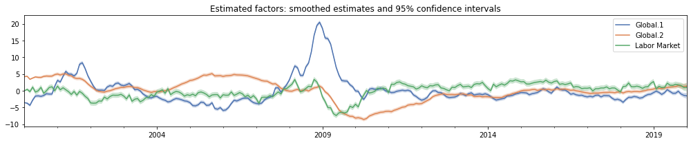
As an example, in the next cell we plot three of the smoothed factors and 95% confidence intervals.
Note: The estimated factors are not identified without additional assumptions that this model does not impose (see for example Bańbura and Modugno, 2014, for details). As a result, it can be difficult to interpet the factors themselves. (Despite this, the space spanned by the factors is identified, so that forecasting and nowcasting exercises, like those we discuss later, are unambiguous).
For example, in the plot below, the “Global.1” factor increases markedly in 2009, following the global financial crisis. However, many of the factor loadings in the summary above are negative – for example, this is true of the output, consumption, and income series. Therefore the increase in the “Global.1” factor during this period actually implies a strong decrease in output, consumption, and income.
# Get estimates of the global and labor market factors,
# conditional on the full dataset ("smoothed")
factor_names = ['Global.1', 'Global.2', 'Labor Market']
mean = results.factors.smoothed[factor_names]

# Compute 95% confidence intervals
from scipy.stats import norm
std = pd.concat([results.factors.smoothed_cov.loc[name, name]
                 for name in factor_names], axis=1)
crit = norm.ppf(1 - 0.05 / 2)
lower = mean - crit * std
upper = mean + crit * std

with sns.color_palette('deep'):
    fig, ax = plt.subplots(figsize=(14, 3))
    mean.plot(ax=ax)

    for name in factor_names:
        ax.fill_between(mean.index, lower[name], upper[name], alpha=0.3)

    ax.set(title='Estimated factors: smoothed estimates and 95% confidence intervals')
    fig.tight_layout();
Explanatory power of the factors
One way to examine how the factors relate to the observed variables is to compute the explanatory power that each factor has for each variable, by regressing each variable on a constant plus one or more of the smoothed factor estimates and storing the resulting $R^2$, or “coefficient of determination”, value.
Computing $R^2$
The get_coefficients_of_determination method in the results object has three options for the method argument:
method='individual'retrieves the $R^2$ value for each observed variable regressed on each individual factor (plus a constant term)method='joint'retrieves the $R^2$ value for each observed variable regressed on all factors that the variable loads onmethod='cumulative'retrieves the $R^2$ value for each observed variable regressed on an expanding set of factors. The expanding set begins with the $R^2$ from a regression of each variable on the first factor that the variable loads on (as it appears in, for example, the summary tables above) plus a constant. For the next factor in the list, the $R^2$ is computed by a regression on the first two factors (assuming that a given variable loads on both factors).
Example: top 10 variables explained by the global factors
Below, we compute according to the method='individual' approach, and then show the top 10 observed variables that are explained (individually) by each of the two global factors.
- The first global factor explains labor market series well, but also includes Real GDP and a measure of stock market volatility (VXO)
- The second factor appears to largely explain housing-related variables (in fact, this might be an argument for dropping the “Housing” group-specific factor)
rsquared = results.get_coefficients_of_determination(method='individual')

top_ten = []
for factor_name in rsquared.columns[:2]:
    top_factor = (rsquared[factor_name].sort_values(ascending=False)
                                       .iloc[:10].round(2).reset_index())
    top_factor.columns = pd.MultiIndex.from_product([
        [f'Top ten variables explained by {factor_name}'],
        ['Variable', r'$R^2$']])
    top_ten.append(top_factor)
pd.concat(top_ten, axis=1)
| Top ten variables explained by Global.1 | Top ten variables explained by Global.2 | |||
|---|---|---|---|---|
| Variable | $R^2$ | Variable | $R^2$ | |
| 0 | All Employees: Total nonfarm | 0.74 | Housing Starts: Total New Privately Owned | 0.65 |
| 1 | All Employees: Goods-Producing Industries | 0.73 | New Private Housing Permits, South (SAAR) | 0.65 |
| 2 | All Employees: Durable goods | 0.66 | Housing Starts, South | 0.65 |
| 3 | All Employees: Manufacturing | 0.65 | New Private Housing Permits (SAAR) | 0.65 |
| 4 | All Employees: Wholesale Trade | 0.64 | New Private Housing Permits, West (SAAR) | 0.64 |
| 5 | All Employees: Service-Providing Industries | 0.63 | Housing Starts, West | 0.64 |
| 6 | All Employees: Trade, Transportation & Utilities | 0.61 | New Private Housing Permits, Midwest (SAAR) | 0.56 |
| 7 | VXO | 0.61 | New Private Housing Permits, Northeast (SAAR) | 0.54 |
| 8 | Real Gross Domestic Product, 3 Decimal (Billio... | 0.53 | Housing Starts, Midwest | 0.52 |
| 9 | All Employees: Construction | 0.52 | Housing Starts, Northeast | 0.52 |
Plotting $R^2$
When there are a large number of observed variables, it is often easier to plot the $R^2$ values for each variable. This can be done using the plot_coefficients_of_determination method in the results object. It accepts the same method arguments as the get_coefficients_of_determination method, above.
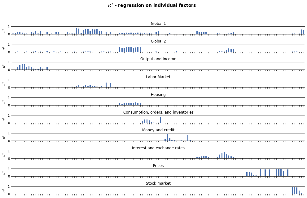
Below, we plot the $R^2$ values from the “individual” regressions, for each factor. Because there are so many variables, this graphical tool is best for identifying trends overall and within groups, and we do not display the names of the variables on the x-axis label.
with sns.color_palette('deep'):
    fig = results.plot_coefficients_of_determination(method='individual', figsize=(14, 9))
    fig.suptitle(r'$R^2$ - regression on individual factors', fontsize=14, fontweight=600)
    fig.tight_layout(rect=[0, 0, 1, 0.95]);
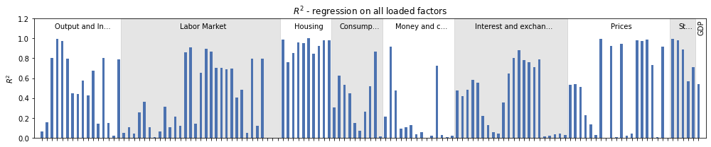
Alternatively, we might look at the overall explanatory value to a given variable of all factors that the variable loads on. To do that, we can use the same function but with method='joint' .
To make it easier to identify patterns, we add in shading and labels to identify the different groups of variables, as well as our only quarterly variable, GDP.
group_counts = defn_m[['description', 'group']]
group_counts = group_counts[group_counts['description'].isin(dta['2020-02'].dta_m.columns)]
group_counts = group_counts.groupby('group', sort=False).count()['description'].cumsum()

with sns.color_palette('deep'):
    fig = results.plot_coefficients_of_determination(method='joint', figsize=(14, 3));

    # Add in group labels
    ax = fig.axes[0]
    ax.set_ylim(0, 1.2)
    for i in np.arange(1, len(group_counts), 2):
        start = 0 if i == 0 else group_counts[i - 1]
        end = group_counts[i] + 1
        ax.fill_between(np.arange(start, end) - 0.6, 0, 1.2, color='k', alpha=0.1)
    for i in range(len(group_counts)):
        start = 0 if i == 0 else group_counts[i - 1]
        end = group_counts[i]
        n = end - start
        text = group_counts.index[i]
        if len(text) > n:
            text = text[:n - 3] + '...'

        ax.annotate(text, (start + n / 2, 1.1), ha='center')

    # Add label for GDP
    ax.set_xlim(-1.5, model.k_endog + 0.5)
    ax.annotate('GDP', (model.k_endog - 1.1, 1.05), ha='left', rotation=90)

    fig.tight_layout();
Forecasting
One of the benefits of these models is that we can use the dynamics of the factors to produce forecasts of any of the observed variables. This is straightforward here, using the forecast or get_forecast results methods. These take a single argument, which must be either:
- an integer, specifying the number of steps ahead to forecast
- a date, specifying the date of the final forecast to make
The forecast method only produces a series of point forecasts for all of the observed variables, while the get_forecast method returns a new forecast results object, that can also be used to compute confidence intervals.
Note: these forecasts are in the same scale as the variables passed to the DynamicFactorMQ constructor, even if standardize=True has been used.
Below is an example of the forecast method.
# Create point forecasts, 3 steps ahead
point_forecasts = results.forecast(steps=3)

# Print the forecasts for the first 5 observed variables
print(point_forecasts.T.head())
                                                2020-02   2020-03   2020-04
Real Personal Income                           0.220708  0.271456  0.257587
Real personal income ex transfer receipts      0.232887  0.270109  0.255253
IP Index                                       0.251309  0.156593  0.161717
IP: Final Products and Nonindustrial Supplies  0.274381  0.113899  0.134390
IP: Final Products (Market Group)              0.279685  0.097909  0.128986
In addition to forecast and get_forecast, there are two more general methods, predict and get_prediction that allow for both of in-sample prediction and out-of-sample forecasting. Instead of a steps argument, they take start and end arguments, which can be either in-sample dates or out-of-sample dates.
Below, we give an example of using get_prediction to show in-sample predictions and out-of-sample forecasts for some spreads between Treasury securities and the Federal Funds Rate.
# Create forecasts results objects, through the end of 20201
prediction_results = results.get_prediction(start='2000', end='2022')

variables = ['1-Year Treasury C Minus FEDFUNDS',
             '5-Year Treasury C Minus FEDFUNDS',
             '10-Year Treasury C Minus FEDFUNDS']

# The `predicted_mean` attribute gives the same
# point forecasts that would have been returned from
# using the `predict` or `forecast` methods.
point_predictions = prediction_results.predicted_mean[variables]

# We can use the `conf_int` method to get confidence
# intervals; here, the 95% confidence interval
ci = prediction_results.conf_int(alpha=0.05)
lower = ci[[f'lower {name}' for name in variables]]
upper = ci[[f'upper {name}' for name in variables]]

# Plot the forecasts and confidence intervals
with sns.color_palette('deep'):
    fig, ax = plt.subplots(figsize=(14, 4))

    # Plot the in-sample predictions
    point_predictions.loc[:'2020-01'].plot(ax=ax)

    # Plot the out-of-sample forecasts
    point_predictions.loc['2020-01':].plot(ax=ax, linestyle='--',
                                           color=['C0', 'C1', 'C2'],
                                           legend=False)

    # Confidence intervals
    for name in variables:
        ax.fill_between(ci.index,
                        lower[f'lower {name}'],
                        upper[f'upper {name}'], alpha=0.1)

    # Forecast period, set title
    ylim = ax.get_ylim()
    ax.vlines('2020-01', ylim[0], ylim[1], linewidth=1)
    ax.annotate(r' Forecast $\rightarrow$', ('2020-01', -1.7))
    ax.set(title=('Treasury securities / Federal Funds Rate spreads:'
                  ' in-sample predictions and out-of-sample forecasts, with 95% confidence intervals'), ylim=ylim)

    fig.tight_layout()
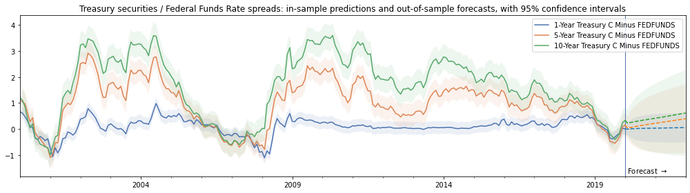
Forecasting example
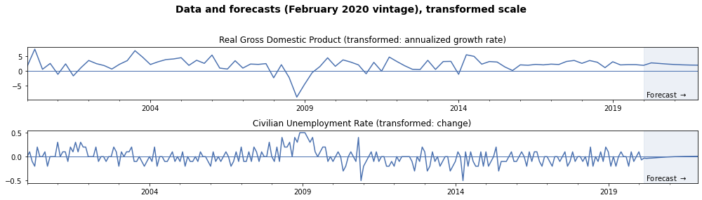
The variables that we showed in the forecasts above were not transformed from their original values. As a result, the predictions were already interpretable as spreads. For the other observed variables that were transformed prior to construting the model, our forecasts will be in the transformed scale.
For example, although the original data in the FRED-MD/QD datasets for Real GDP is in “Billions of Chained 2012 Dollars”, this variable was transformed to the annualized quarterly growth rate (percent change) for inclusion in the model. Similarly, the Civilian Unemployment Rate was originally in “Percent”, but it was transformed into the 1-month change (first difference) for inclusion in the model.
Because the transformed data was provided to the model, the prediction and forecasting methods will produce predictions and forecasts in the transformed space. (Reminder: the transformation step, which we did prior to constructing the model, is different from the standardization step, which the model handles automatically, and which we do not need to manually reverse).
Below, we compute and plot the forecasts directly from the model associated with real GDP and the unemployment rate.
# Get the titles of the variables as they appear in the dataset
unemp_description = 'Civilian Unemployment Rate'
gdp_description = 'Real Gross Domestic Product, 3 Decimal (Billions of Chained 2012 Dollars)'

# Compute the point forecasts
fcast_m = results.forecast('2021-12')[unemp_description]
fcast_q = results.forecast('2021-12')[gdp_description].resample('Q').last()
# For more convenient plotting, combine the observed data with the forecasts
plot_m = pd.concat([dta['2020-02'].dta_m.loc['2000':, unemp_description], fcast_m])
plot_q = pd.concat([dta['2020-02'].dta_q.loc['2000':, gdp_description], fcast_q])

with sns.color_palette('deep'):
    fig, axes = plt.subplots(2, figsize=(14, 4))

    # Plot real GDP growth, data and forecasts
    plot_q.plot(ax=axes[0])
    axes[0].set(title='Real Gross Domestic Product (transformed: annualized growth rate)')
    axes[0].hlines(0, plot_q.index[0], plot_q.index[-1], linewidth=1)

    # Plot the change in the unemployment rate, data and forecasts
    plot_m.plot(ax=axes[1])
    axes[1].set(title='Civilian Unemployment Rate (transformed: change)')
    axes[1].hlines(0, plot_m.index[0], plot_m.index[-1], linewidth=1)

    # Show the forecast period in each graph
    for i in range(2):
        ylim = axes[i].get_ylim()
        axes[i].fill_between(plot_q.loc['2020-02':].index,
                             ylim[0], ylim[1], alpha=0.1, color='C0')
        axes[i].annotate(r' Forecast $\rightarrow$',
                         ('2020-03', ylim[0] + 0.1 * ylim[1]))
        axes[i].set_ylim(ylim)

    # Title
    fig.suptitle('Data and forecasts (February 2020 vintage), transformed scale',
                 fontsize=14, fontweight=600)

    fig.tight_layout(rect=[0, 0, 1, 0.95]);
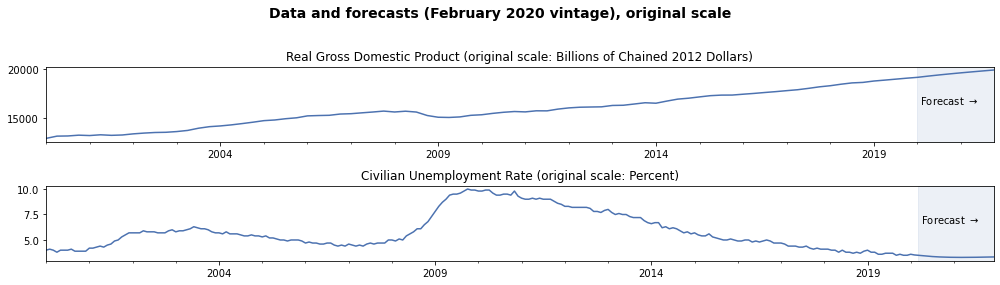
For point forecasts, we can also reverse the transformations to get point forecasts in the original scale.
Aside: for non-linear transformations, it would not be valid to compute confidence intervals in the original space by reversing the transformation on the confidence intervals computed for the transformed space.
# Reverse the transformations

# For real GDP, we take the level in 2000Q1 from the original data,
# and then apply the growth rates to compute the remaining levels
plot_q_orig = (plot_q / 100 + 1)**0.25
plot_q_orig.loc['2000Q1'] = dta['2020-02'].orig_q.loc['2000Q1', gdp_description]
plot_q_orig = plot_q_orig.cumprod()

# For the unemployment rate, we take the level in 2000-01 from
# the original data, and then we apply the changes to compute the
# remaining levels
plot_m_orig = plot_m.copy()
plot_m_orig.loc['2000-01'] = dta['2020-02'].orig_m.loc['2000-01', unemp_description]
plot_m_orig = plot_m_orig.cumsum()
with sns.color_palette('deep'):
    fig, axes = plt.subplots(2, figsize=(14, 4))

    # Plot real GDP, data and forecasts
    plot_q_orig.plot(ax=axes[0])
    axes[0].set(title=('Real Gross Domestic Product'
                       ' (original scale: Billions of Chained 2012 Dollars)'))

    # Plot the unemployment rate, data and forecasts
    plot_m_orig.plot(ax=axes[1])
    axes[1].set(title='Civilian Unemployment Rate (original scale: Percent)')

    # Show the forecast period in each graph
    for i in range(2):
        ylim = axes[i].get_ylim()
        axes[i].fill_between(plot_q.loc['2020-02':].index,
                             ylim[0], ylim[1], alpha=0.1, color='C0')
        axes[i].annotate(r' Forecast $\rightarrow$',
                         ('2020-03', ylim[0] + 0.5 * (ylim[1] - ylim[0])))
        axes[i].set_ylim(ylim)

    # Title
    fig.suptitle('Data and forecasts (February 2020 vintage), original scale',
                 fontsize=14, fontweight=600)

    fig.tight_layout(rect=[0, 0, 1, 0.95]);
Nowcasting GDP, real-time forecast updates, and the news
The forecasting exercises above were based on our baseline results object, which was computed using the February 2020 vintage of data. This was prior to any effect from the COVID-19 pandemic, and near the end of a historically long economic expansion. As a result, the forecasts above paint a relatively rosy picture for the economy, with strong real GDP growth and a continued decline in the unemployment rate. However, the economic data for March through June (which is the last vintage that was available at the time this notebook was produced) showed strong negative economic effects stemming from the pandemic and the associated disruptions to economic activity.
It is straightforward to update our model to take into account new data, and to produce new forecasts. Moreover, we can compute the effect that each new observation has on our forecasts. To illustrate, we consider the exercise of forecasting real GDP growth in 2020Q2. Since this is the current quarter for most of this period, this is an example of “nowcasting”.
Baseline GDP forecast: February 2020 vintage
To begin with, we examine the forecast of our model for real GDP growth in 2020Q2. This model is a mixed frequency model that is estimated at the monthly frequency, and the estimates for quarterly variables correspond to the last months of each quarter. As a result, we’re interested in the forecast for June 2020.
# The original point forecasts are monthly
point_forecasts_m = results.forecast('June 2020')[gdp_description]

# Resample to quarterly frequency by taking the value in the last
# month of each quarter
point_forecasts_q = point_forecasts_m.resample('Q').last()

print('Baseline (February 2020) forecast for real GDP growth'
      f' in 2020Q2: {point_forecasts_q["2020Q2"]:.2f}%')
Baseline (February 2020) forecast for real GDP growth in 2020Q2: 2.68%
Updated GDP forecast: March 2020 vintage
Next, we consider taking into account data for the next available vintage, which is March 2020. Note that for the March 2020 vintage, the reference month of the released data still only covers the period through February 2020. This is still before the economic effects of the pandemic, so we expect to see only minor changes to our forecast.
For simplicity, in this exercise we will not be re-estimating the model parameters with the updated data, although that is certainly possible.
There are a variety of methods in the results object that make it easy to extend the model with new data or even apply a given model to an entirely different dataset. They are append, extend, and apply. For more details about these methods, see this example notebook.
Here, we will use the apply method, which applies the model and estimated parameters to a new dataset.
Notes:
- If
standardize=Truewas used in model creation (which is the default), then theapplymethod will use the same standardization on the new dataset as on the original dataset by default. This is important when exploring the impacts of the “news”, as we will be doing, and it is another reason that it is usually easiest to leave standardization to the model (if you prefer to re-standardize the new dataset, you can use theretain_standardization=Falseargument to theapplymethod). - Because of the fact that some data in the FRED-MD dataset is revised after its initial publication, we are not just adding new observations but are potentially changing the values of previously observed entries (this is why we need to use the
applymethod rather than theappendmethod).
# Since we will be collecting results for a number of vintages,
# construct a dictionary to hold them, and include the baseline
# results from February 2020
vintage_results = {'2020-02': results}

# Get the updated monthly and quarterly datasets
start = '2000'
updated_endog_m = dta['2020-03'].dta_m.loc[start:, :]
gdp_description = defn_q.loc['GDPC1', 'description']
updated_endog_q = dta['2020-03'].dta_q.loc[start:, [gdp_description]]

# Get the results for March 2020 using `apply`
vintage_results['2020-03'] = results.apply(
    updated_endog_m, endog_quarterly=updated_endog_q)
This new results object has all of the same attributes and methods as the baseline results object. For example, we can compute the updated forecast for real GDP growth in 2020Q2.
# Print the updated forecast for real GDP growth in 2020Q2
updated_forecasts_q = (
    vintage_results['2020-03'].forecast('June 2020')[gdp_description]
                              .resample('Q').last())

print('March 2020 forecast for real GDP growth in 2020Q2:'
      f' {updated_forecasts_q["2020Q2"]:.2f}%')
March 2020 forecast for real GDP growth in 2020Q2: 2.52%
As expected, the forecast from March 2020 is only a little changed from our baseline (February 2020) forecast.
We can continue this process, however, for the April, May, and June vintages and see how the incoming economic data changes our forecast for real GDP.
# Apply our results to the remaining vintages
for vintage in ['2020-04', '2020-05', '2020-06']:
    # Get updated data for the vintage
    updated_endog_m = dta[vintage].dta_m.loc[start:, :]
    updated_endog_q = dta[vintage].dta_q.loc[start:, [gdp_description]]

    # Get updated results for for the vintage
    vintage_results[vintage] = results.apply(
        updated_endog_m, endog_quarterly=updated_endog_q)
# Compute forecasts for each vintage
forecasts = {vintage: res.forecast('June 2020')[gdp_description]
                         .resample('Q').last().loc['2020Q2']
             for vintage, res in vintage_results.items()}
# Convert to a Pandas series with a date index
forecasts = pd.Series(list(forecasts.values()),
                      index=pd.PeriodIndex(forecasts.keys(), freq='M'))

# Print our forecast for 2020Q2 real GDP growth across all vintages
for vintage, value in forecasts.items():
    print(f'{vintage} forecast for real GDP growth in 2020Q2:'
          f' {value:.2f}%')
2020-02 forecast for real GDP growth in 2020Q2: 2.68%
2020-03 forecast for real GDP growth in 2020Q2: 2.52%
2020-04 forecast for real GDP growth in 2020Q2: -8.23%
2020-05 forecast for real GDP growth in 2020Q2: -37.17%
2020-06 forecast for real GDP growth in 2020Q2: -22.33%
Although there was not much of a change in the forecast between the February and March vintages, the forecasts from the April and May vintages each saw substantial declines.
To dig into why the forecast changed so much, we can compute the impacts on the forecast of each piece of new information in each of the data updates. This computation of the “news” and its impact on forecasts follows Bańbura and Modugno (2014).
Computation of the “news” and the associated impact is straightforward using the news method of the results object associated with one of the vintages. The basic syntax is:
results.news(previous_vintage_results, impact_date='2020-06',
             impacted_variable=gdp_description,
             comparison_type='previous')
The “news” is then unexpected component of the updated datapoints in results that were not present in the previous_vintage_results, and the impacts will be computed for forecasts related to June 2020 (recall that for the mixed frequency setup here, the quarterly values are identified with the last monthly value in each quarter). This method returns a new results object, with a number of tables that decompose the impacts in variety of ways. For additional details about the computation of the “news” and the associated impacts, see this example notebook.
As an example, we will examine the news and impacts associated with the April 2020 vintage, compared to the March 2020 vintage.
# Compute the news and impacts on the real GDP growth forecast
# for 2020Q2, between the April and March vintages
news = vintage_results['2020-04'].news(
    vintage_results['2020-03'], impact_date='2020-06',
    impacted_variable=gdp_description,
    comparison_type='previous')

# The `summary` method summarizes all updates. Here we aren't
# showing it, to save space.
# news.summary()
Details of impacts: April vintage compared to March vintage
Now, we will show which ten new observations had the largest impact (in absolute value) on the forecast of real GDP growth in 2020Q2. This is shown in the table below, which has seven columns:
- The first column, “update date”, is the date of the new observation.
- The second column, “updated variable”, is the variable updated
- The third column, “observed”, shows the actual recorded value
- The fourth column, “forecast (prev)”, shows what value had been expected in the previous vintage (here, in the March 2020 vintage).
- The fifth column, “news”, shows the unexpected component of the update (it is equal to observed - forecast (prev))
- The sixth column, “weight”, shows how much weight this date / variable combination has on the forecast of interest
- The final column, “impact”, shows how much the forecast of real GDP growth in 2020Q2 changed based only on the single new observation captured by each given row
From this table, we can see that in the April vintage, the largest impacts on the real GDP forecast for 2020Q2 came from:
- Initial unemployment claims and the CBOE S&P 100 Volatility Index (VXO) each came in much higher than expected
- Corporate bond spreads (AAA and BAA) came in higher than expected
- Industrial production (including final products, manufacturing, durable materials, and the overall index) and capcity utilization came in much lower than expected
# We can re-arrange the `details_by_impact` table to show the new
# observations with the top ten impacts (in absolute value)
details = news.details_by_impact
details.index = details.index.droplevel(['impact date', 'impacted variable'])
details['absolute impact'] = np.abs(details['impact'])
details = (details.sort_values('absolute impact', ascending=False)
                  .drop('absolute impact', axis=1))
details.iloc[:10].round(2)
| observed | forecast (prev) | news | weight | impact | ||
|---|---|---|---|---|---|---|
| update date | updated variable | |||||
| 2020-03 | IP: Final Products and Nonindustrial Supplies | -6.53 | -0.11 | -6.42 | 0.61 | -3.92 |
| Initial Claims | 253.49 | 0.94 | 252.54 | -0.01 | -2.06 | |
| Moody’s Baa Corporate Bond Minus FEDFUNDS | 3.66 | 2.10 | 1.56 | -0.63 | -0.99 | |
| IP: Final Products (Market Group) | -6.52 | -0.12 | -6.39 | -0.13 | 0.84 | |
| VXO | 63.88 | 19.53 | 44.35 | -0.01 | -0.60 | |
| IP: Manufacturing (SIC) | -6.46 | 0.05 | -6.50 | 0.06 | -0.40 | |
| Moody’s Aaa Corporate Bond Minus FEDFUNDS | 2.39 | 1.25 | 1.14 | -0.35 | -0.40 | |
| IP: Consumer Goods | -6.06 | -0.21 | -5.84 | -0.07 | 0.39 | |
| All Employees: Total nonfarm | -0.46 | 0.15 | -0.61 | 0.53 | -0.32 | |
| 6-Month Treasury Bill: | -1.18 | -0.06 | -1.12 | 0.27 | -0.30 |
For each updated vintage of data, we can compute the news in the same way. Below, we compute all news vintages.
news_results = {}
vintages = ['2020-02', '2020-03', '2020-04', '2020-05', '2020-06']
impact_date = '2020-06'

for i in range(1, len(vintages)):
    vintage = vintages[i]
    prev_vintage = vintages[i - 1]

    # Notice that to get the "incremental" news, we are computing
    # the news relative to the previous vintage and not to the baseline
    # (February 2020) vintage
    news_results[vintage] = vintage_results[vintage].news(
        vintage_results[prev_vintage],
        impact_date=impact_date,
        impacted_variable=gdp_description,
        comparison_type='previous')
Impacts by group: evolution across all vintages
To summarize the news, we will take an approach similar to that of the New York Fed Staff Nowcast, and combine impacts by the groups defined above (for example “Output and Income”, etc.).
Note: the New York Fed Staff Nowcast uses precisely the same dynamic factor model and estimation rountine (EM algorithm) to compute their nowcast, although they use a different dataset and different factor specification. In addition, they update their dataset and forecast every week, while the FRED-MD dataset we’re using here only updates every month.
group_impacts = {'2020-02': None}

for vintage, news in news_results.items():
    # Start from the details by impact table
    details_by_impact = (
        news.details_by_impact.reset_index()
            .drop(['impact date', 'impacted variable'], axis=1))

    # Merge with the groups dataset, so that we can identify
    # which group each individual impact belongs to
    impacts = (pd.merge(details_by_impact, groups, how='left',
                        left_on='updated variable', right_on='description')
                 .drop('description', axis=1)
                 .set_index(['update date', 'updated variable']))

    # Compute impacts by group, summing across the individual impacts
    group_impacts[vintage] = impacts.groupby('group').sum()['impact']

# Add in a row of zeros for the baseline forecast
group_impacts['2020-02'] = group_impacts['2020-03'] * np.nan

# Convert into a Pandas DataFrame, and fill in missing entries
# with zeros (missing entries happen when there were no updates
# for a given group in a given vintage)
group_impacts = (
    pd.concat(group_impacts, axis=1)
      .fillna(0)
      .reindex(group_counts.index).T)
group_impacts.index = forecasts.index

# Print the table of impacts from data in each group,
# along with a row with the "Total" impact
(group_impacts.T
    .append(group_impacts.sum(axis=1).rename('Total impact on 2020Q2 forecast'))
    .round(2).iloc[:, 1:])
| 2020-03 | 2020-04 | 2020-05 | 2020-06 | |
|---|---|---|---|---|
| group | ||||
| Output and Income | -0.12 | -3.85 | -10.08 | 9.15 |
| Labor Market | 0.29 | -3.38 | -19.76 | 5.94 |
| Housing | -0.09 | -0.05 | -0.00 | 0.26 |
| Consumption, orders, and inventories | -0.04 | -0.39 | -0.35 | 0.47 |
| Money and credit | -0.02 | -0.01 | -0.08 | 0.05 |
| Interest and exchange rates | -0.13 | -2.67 | 0.94 | 0.97 |
| Prices | 0.00 | 0.01 | 0.00 | 0.00 |
| Stock market | -0.05 | -0.35 | 0.02 | 0.33 |
| Total impact on 2020Q2 forecast | -0.16 | -10.70 | -29.30 | 17.18 |
Impacts by group: graphical illustration
While the table is informative, a graphical version can be even more helpful. Below, we show a figure of the type shown in Bańbura and Modugno (2014), but also used in, for example, the New York Fed Staff Nowcast.
with sns.color_palette('deep'):
    fig, ax = plt.subplots(figsize=(14, 6))

    # Stacked bar plot showing the impacts by group
    group_impacts.plot(kind='bar', stacked=True, width=0.3, zorder=2, ax=ax);

    # Line plot showing the forecast for real GDP growth in 2020Q2 for each vintage
    x = np.arange(len(forecasts))
    ax.plot(x, forecasts, marker='o', color='k', markersize=7, linewidth=2)
    ax.hlines(0, -1, len(group_impacts) + 1, linewidth=1)

    # x-ticks
    labels = group_impacts.index.strftime('%b')
    ax.xaxis.set_ticklabels(labels)
    ax.xaxis.set_tick_params(size=0)
    ax.xaxis.set_tick_params(labelrotation='auto', labelsize=13)

    # y-ticks
    ax.yaxis.set_tick_params(direction='in', size=0, labelsize=13)
    ax.yaxis.grid(zorder=0)

    # title, remove spines
    ax.set_title('Evolution of real GDP growth nowcast: 2020Q2', fontsize=16, fontweight=600, loc='left')
    [ax.spines[spine].set_visible(False)
     for spine in ['top', 'left', 'bottom', 'right']]

    # base forecast vs updates
    ylim = ax.get_ylim()
    ax.vlines(0.5, ylim[0], ylim[1] + 5, linestyles='--')
    ax.annotate('Base forecast', (-0.2, 22), fontsize=14)
    ax.annotate(r'Updated forecasts and impacts from the "news" $\rightarrow$', (0.65, 22), fontsize=14)

    # legend
    ax.legend(loc='upper center', ncol=4, fontsize=13, bbox_to_anchor=(0.5, -0.1), frameon=False)

    fig.tight_layout();
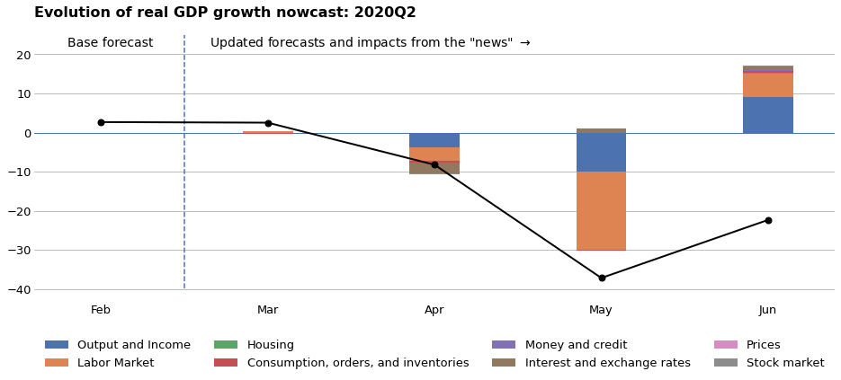
References
Bańbura, Marta, and Michele Modugno. “Maximum likelihood estimation of factor models on datasets with arbitrary pattern of missing data.” Journal of Applied Econometrics 29, no. 1 (2014): 133-160.
Bańbura, Marta, Domenico Giannone, and Lucrezia Reichlin. “Nowcasting.” The Oxford Handbook of Economic Forecasting. July 8, 2011.
Bok, Brandyn, Daniele Caratelli, Domenico Giannone, Argia M. Sbordone, and Andrea Tambalotti. 2018. “Macroeconomic Nowcasting and Forecasting with Big Data.” Annual Review of Economics 10 (1): 615-43.
Mariano, Roberto S., and Yasutomo Murasawa. “A coincident index, common factors, and monthly real GDP.” Oxford Bulletin of Economics and Statistics 72, no. 1 (2010): 27-46.
McCracken, Michael W., and Serena Ng. “FRED-MD: A monthly database for macroeconomic research.” Journal of Business & Economic Statistics 34, no. 4 (2016): 574-589.