Implementing and estimating an ARMA(1, 1) state space model(Open on Google Colab | View / download notebook | Report a problem)
This notebook collects the full example implementing and estimating (via maximum likelihood, Metropolis-Hastings, and Gibbs Sampling) a specific autoregressive integrated moving average (ARIMA) model, from my working paper Estimating time series models by state space methods in Python: Statsmodels.
Table of Contents
ARMA(1, 1) - CPI Inflation
This notebook contains the example code from “State Space Estimation of Time Series Models in Python: Statsmodels” for the ARMA(1, 1) model of CPI inflation.
# These are the basic import statements to get the required Python functionality
%matplotlib inline

import numpy as np
import pandas as pd
import statsmodels.api as sm
import matplotlib.pyplot as plt
Data
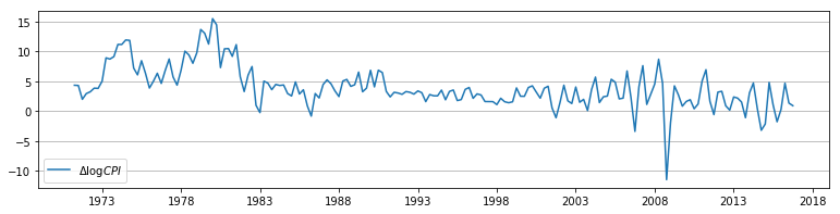
For this example, we consider modeling quarterly CPI inflation. Below, we retrieve the data directly from the Federal Reserve Economic Database using the pandas_datareader package.
# Get the data from FRED
from pandas_datareader.data import DataReader
cpi = DataReader('CPIAUCNS', 'fred', start='1971-01', end='2016-12')
cpi.index = pd.DatetimeIndex(cpi.index, freq='MS')
inf = np.log(cpi).resample('QS').mean().diff()[1:] * 400

# Plot the series to see what it looks like
fig, ax = plt.subplots(figsize=(13, 3), dpi=300)
ax.plot(inf.index, inf, label=r'$\Delta \log CPI$')
ax.legend(loc='lower left')
ax.yaxis.grid();
State space model
The ARMA(1, 1) model is:
\[y_t = \phi y_{t-1} + \varepsilon_t + \theta_1 \varepsilon_{t-1}, \qquad \varepsilon_t \sim N(0, \sigma^2)\]and it can be written in state-space form as:
\[\begin{align} y_t & = \underbrace{\begin{bmatrix} 1 & \theta_1 \end{bmatrix}}_{Z} \underbrace{\begin{bmatrix} \alpha_{1,t} \\ \alpha_{2,t} \end{bmatrix}}_{\alpha_t} \\ \begin{bmatrix} \alpha_{1,t+1} \\ \alpha_{2,t+1} \end{bmatrix} & = \underbrace{\begin{bmatrix} \phi & 0 \\ 1 & 0 \\ \end{bmatrix}}_{T} \begin{bmatrix} \alpha_{1,t} \\ \alpha_{2,t} \end{bmatrix} + \underbrace{\begin{bmatrix} 1 \\ 0 \end{bmatrix}}_{R} \underbrace{\varepsilon_{t+1}}_{\eta_t} \\ \end{align}\]Below we construct a custom class, ARMA11, to estimate the ARMA(1, 1) model.
from statsmodels.tsa.statespace.tools import (constrain_stationary_univariate,
                                              unconstrain_stationary_univariate)

class ARMA11(sm.tsa.statespace.MLEModel):
    start_params = [0, 0, 1]
    param_names = ['phi', 'theta', 'sigma2']

    def __init__(self, endog):
        super(ARMA11, self).__init__(
            endog, k_states=2, k_posdef=1, initialization='stationary')

        self['design', 0, 0] = 1.
        self['transition', 1, 0] = 1.
        self['selection', 0, 0] = 1.

    def transform_params(self, params):
        phi = constrain_stationary_univariate(params[0:1])
        theta = constrain_stationary_univariate(params[1:2])
        sigma2 = params[2]**2
        return np.r_[phi, theta, sigma2]

    def untransform_params(self, params):
        phi = unconstrain_stationary_univariate(params[0:1])
        theta = unconstrain_stationary_univariate(params[1:2])
        sigma2 = params[2]**0.5
        return np.r_[phi, theta, sigma2]

    def update(self, params, **kwargs):
        # Transform the parameters if they are not yet transformed
        params = super(ARMA11, self).update(params, **kwargs)

        self['design', 0, 1] = params[1]
        self['transition', 0, 0] = params[0]
        self['state_cov', 0, 0] = params[2]
Maximum likelihood estimation
With this class, we can instantiate a new object with the inflation data and fit the model by maximum likelihood methods.
inf_model = ARMA11(inf)
inf_results = inf_model.fit()

print(inf_results.summary())
                           Statespace Model Results
==============================================================================
Dep. Variable:               CPIAUCNS   No. Observations:                  183
Model:                         ARMA11   Log Likelihood                -432.375
Date:                Sat, 28 Jan 2017   AIC                            870.750
Time:                        09:34:31   BIC                            880.379
Sample:                    04-01-1971   HQIC                           874.653
                         - 10-01-2016
Covariance Type:                  opg
==============================================================================
                 coef    std err          z      P>|z|      [0.025      0.975]
------------------------------------------------------------------------------
phi            0.9784      0.016     62.713      0.000       0.948       1.009
theta         -0.6338      0.059    -10.750      0.000      -0.749      -0.518
sigma2         6.5407      0.342     19.145      0.000       5.871       7.210
===================================================================================
Ljung-Box (Q):                      258.37   Jarque-Bera (JB):               653.28
Prob(Q):                              0.00   Prob(JB):                         0.00
Heteroskedasticity (H):               1.77   Skew:                            -1.48
Prob(H) (two-sided):                  0.03   Kurtosis:                        11.77
===================================================================================

Warnings:
[1] Covariance matrix calculated using the outer product of gradients (complex-step).
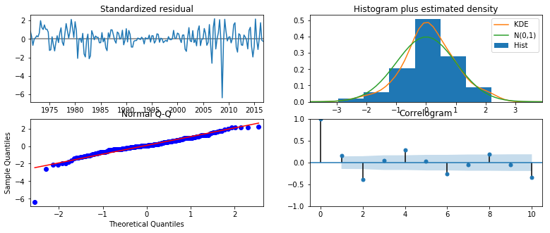
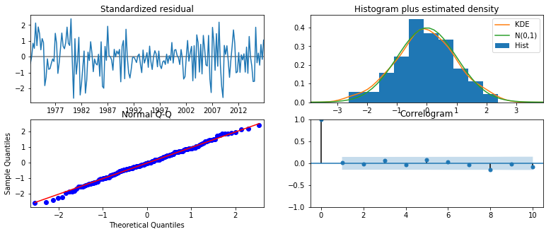
Notice that the diagnostic tests reported in the lower table suggest that our residuals do not appear to be white noise - in particular, we can reject at the 5% level the null hypotheses of serial independence (Ljung-Box test), homoskedasticity (Heteroskedasticity test), and normality (Jarque-Bera test).
To further investicate the residuals, we can produce diagnostic plots.
inf_results.plot_diagnostics(figsize=(13, 5));
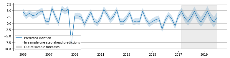
We can also produce in-sample one-step-ahead predictions and out-of-sample forecasts:
# Construct the predictions / forecasts
inf_forecast = inf_results.get_prediction(start='2005-01-01', end='2020-01-01')

# Plot them
fig, ax = plt.subplots(figsize=(13, 3), dpi=300)

forecast = inf_forecast.predicted_mean
ci = inf_forecast.conf_int(alpha=0.5)

ax.fill_between(forecast.ix['2017-01-02':].index, -3, 7, color='grey',
                alpha=0.15)
lines, = ax.plot(forecast.index, forecast)
ax.fill_between(forecast.index, ci['lower CPIAUCNS'], ci['upper CPIAUCNS'],
                alpha=0.2)

p1 = plt.Rectangle((0, 0), 1, 1, fc="white")
p2 = plt.Rectangle((0, 0), 1, 1, fc="grey", alpha=0.3)
ax.legend([lines, p1, p2], ["Predicted inflation",
                            "In-sample one-step-ahead predictions",
                            "Out-of-sample forecasts"], loc='upper left')
ax.yaxis.grid()
And we can produce impulse responses.
# Construct the impulse responses
inf_irfs = inf_results.impulse_responses(steps=10)

print(inf_irfs)
0     1.000000
1     0.344649
2     0.337211
3     0.329933
4     0.322812
5     0.315845
6     0.309028
7     0.302358
8     0.295832
9     0.289447
10    0.283200
Name: CPIAUCNS, dtype: float64
ARMA(1, 1) in Statsmodels via SARIMAX
The large class of seasonal autoregressive integrated moving average models - SARIMAX(p, d, q)x(P, D, Q, S) - is implemented in Statsmodels in the sm.tsa.SARIMAX class.
First, we’ll check that fitting an ARMA(1, 1) model by maximum likelihood using sm.tsa.SARIMAX gives the same results as our ARMA11 class, above.
inf_model2 = sm.tsa.SARIMAX(inf, order=(1, 0, 1))
inf_results2 = inf_model2.fit()

print(inf_results2.summary())
                           Statespace Model Results
==============================================================================
Dep. Variable:               CPIAUCNS   No. Observations:                  183
Model:               SARIMAX(1, 0, 1)   Log Likelihood                -432.375
Date:                Sat, 28 Jan 2017   AIC                            870.750
Time:                        09:42:59   BIC                            880.379
Sample:                    04-01-1971   HQIC                           874.653
                         - 10-01-2016
Covariance Type:                  opg
==============================================================================
                 coef    std err          z      P>|z|      [0.025      0.975]
------------------------------------------------------------------------------
ar.L1          0.9784      0.016     62.707      0.000       0.948       1.009
ma.L1         -0.6337      0.059    -10.749      0.000      -0.749      -0.518
sigma2         6.5408      0.342     19.145      0.000       5.871       7.210
===================================================================================
Ljung-Box (Q):                      258.38   Jarque-Bera (JB):               653.30
Prob(Q):                              0.00   Prob(JB):                         0.00
Heteroskedasticity (H):               1.77   Skew:                            -1.48
Prob(H) (two-sided):                  0.03   Kurtosis:                        11.77
===================================================================================

Warnings:
[1] Covariance matrix calculated using the outer product of gradients (complex-step).
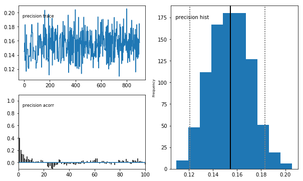
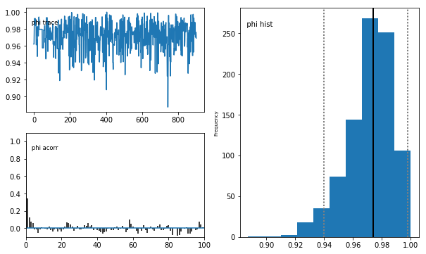
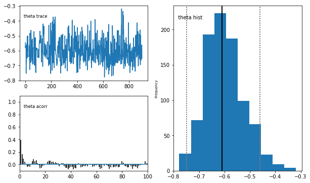
Metropolis-Hastings - ARMA(1, 1)
Here we show how to estimate the ARMA(1, 1) model via Metropolis-Hastings using PyMC. Recall that the ARMA(1, 1) model has three parameters: $(\phi, \theta, \sigma^2)$.
For $\phi$ and $\theta$ we specify uniform priors of $(-1, 1)$, and for $1 / \sigma^2$ we specify a $\Gamma(2, 4)$ prior.
import pymc as mc

# Priors
prior_phi = mc.Uniform('phi', -1, 1)
prior_theta = mc.Uniform('theta', -1, 1)
prior_precision = mc.Gamma('precision', 2, 4)

# Create the model for likelihood evaluation
model = sm.tsa.SARIMAX(inf, order=(1, 0, 1))

# Create the "data" component (stochastic and observed)
@mc.stochastic(dtype=sm.tsa.statespace.MLEModel, observed=True)
def loglikelihood(value=model, phi=prior_phi, theta=prior_theta, precision=prior_precision):
    return value.loglike([phi, theta, 1 / precision])

# Create the PyMC model
pymc_model = mc.Model((prior_phi, prior_theta, prior_precision, loglikelihood))

# Create a PyMC sample and perform sampling
sampler = mc.MCMC(pymc_model)
sampler.sample(iter=10000, burn=1000, thin=10)
[-----------------100%-----------------] 10000 of 10000 complete in 11.7 sec
# Plot traces
mc.Matplot.plot(sampler)
Plotting precision
Plotting phi
Plotting theta
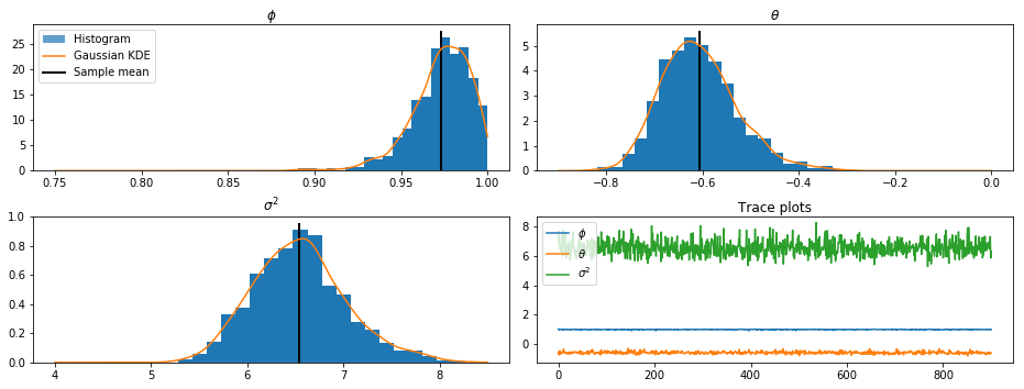
Gibbs Sampling - ARMA(1, 1)
Here we show how to estimate the ARMA(1, 1) model via Metropolis-within-Gibbs Sampling.
from scipy.stats import multivariate_normal, invgamma

def draw_posterior_phi(model, states, sigma2):
    Z = states[0:1, 1:]
    X = states[0:1, :-1]

    tmp = np.linalg.inv(sigma2 * np.eye(1) + np.dot(X, X.T))
    post_mean = np.dot(tmp, np.dot(X, Z.T))
    post_var = tmp * sigma2

    return multivariate_normal(post_mean, post_var).rvs()

def draw_posterior_sigma2(model, states, phi):
    resid = states[0, 1:] - phi * states[0, :-1]
    post_shape = 3 + model.nobs
    post_scale = 3 + np.sum(resid**2)

    return invgamma(post_shape, scale=post_scale).rvs()

np.random.seed(17429)

from scipy.stats import norm, uniform
from statsmodels.tsa.statespace.tools import is_invertible

# Create the model for likelihood evaluation and the simulation smoother
model = ARMA11(inf)
sim_smoother = model.simulation_smoother()

# Create the random walk and comparison random variables
rw_proposal = norm(scale=0.3)

# Create storage arrays for the traces
n_iterations = 10000
trace = np.zeros((n_iterations + 1, 3))
trace_accepts = np.zeros(n_iterations)
trace[0] = [0, 0, 1.]  # Initial values

# Iterations
for s in range(1, n_iterations + 1):
    # 1. Gibbs step: draw the states using the simulation smoother
    model.update(trace[s-1], transformed=True)
    sim_smoother.simulate()
    states = sim_smoother.simulated_state[:, :-1]

    # 2. Gibbs step: draw the autoregressive parameters, and apply
    # rejection sampling to ensure an invertible lag polynomial
    phi = draw_posterior_phi(model, states, trace[s-1, 2])
    while not is_invertible([1, -phi]):
        phi = draw_posterior_phi(model, states, trace[s-1, 2])
    trace[s, 0] = phi

    # 3. Gibbs step: draw the variance parameter
    sigma2 = draw_posterior_sigma2(model, states, phi)
    trace[s, 2] = sigma2

    # 4. Metropolis-step for the moving-average parameter
    theta = trace[s-1, 1]
    proposal = theta + rw_proposal.rvs()
    if proposal > -1 and proposal < 1:
        acceptance_probability = np.exp(
            model.loglike([phi, proposal, sigma2]) -
            model.loglike([phi, theta, sigma2]))

        if acceptance_probability > uniform.rvs():
            theta = proposal
            trace_accepts[s-1] = 1
    trace[s, 1] = theta

# For analysis, burn the first 1000 observations, and only
# take every tenth remaining observation
burn = 1000
thin = 10
final_trace = trace[burn:][::thin]
from scipy.stats import gaussian_kde

fig, axes = plt.subplots(2, 2, figsize=(13, 5), dpi=300)

phi_kde = gaussian_kde(final_trace[:, 0])
theta_kde = gaussian_kde(final_trace[:, 1])
sigma2_kde = gaussian_kde(final_trace[:, 2])

axes[0, 0].hist(final_trace[:, 0], bins=20, normed=True, alpha=1)
X = np.linspace(0.75, 1.0, 5000)
line, = axes[0, 0].plot(X, phi_kde(X))
ylim = axes[0, 0].get_ylim()
vline = axes[0, 0].vlines(final_trace[:, 0].mean(), ylim[0], ylim[1],
                          linewidth=2)
axes[0, 0].set(title=r'$\phi$')

axes[0, 1].hist(final_trace[:, 1], bins=20, normed=True, alpha=1)
X = np.linspace(-0.9, 0.0, 5000)
axes[0, 1].plot(X, theta_kde(X))
ylim = axes[0, 1].get_ylim()
vline = axes[0, 1].vlines(final_trace[:, 1].mean(), ylim[0], ylim[1],
                          linewidth=2)
axes[0, 1].set(title=r'$\theta$')

axes[1, 0].hist(final_trace[:, 2], bins=20, normed=True, alpha=1)
X = np.linspace(4, 8.5, 5000)
axes[1, 0].plot(X, sigma2_kde(X))
ylim = axes[1, 0].get_ylim()
vline = axes[1, 0].vlines(final_trace[:, 2].mean(), ylim[0], ylim[1],
                          linewidth=2)
axes[1, 0].set(title=r'$\sigma^2$')

p1 = plt.Rectangle((0, 0), 1, 1, alpha=0.7)
axes[0, 0].legend([p1, line, vline],
                  ["Histogram", "Gaussian KDE", "Sample mean"],
                  loc='upper left')

axes[1, 1].plot(final_trace[:, 0], label=r'$\phi$')
axes[1, 1].plot(final_trace[:, 1], label=r'$\theta$')
axes[1, 1].plot(final_trace[:, 2], label=r'$\sigma^2$')
axes[1, 1].legend(loc='upper left')
axes[1, 1].set(title=r'Trace plots')
fig.tight_layout()
Expanded model: SARIMAX
We’ll try a more complicated model now: SARIMA(3, 0, 0)x(0, 1, 1, 4). The ability to include a seasonal effect is important, since the data series we selected is not seasonally adjusted.
We also add an explanatory “impulse” variable to account for the clear outlier in the fourth quarter of 2008. We’ll estimate this model by maximum likelihood.
outlier_exog = pd.Series(np.zeros(len(inf)), index=inf.index, name='outlier')
outlier_exog['2008-10-01'] = 1
inf_model3 = sm.tsa.SARIMAX(inf, order=(3, 0, 0), seasonal_order=(0, 1, 1, 4), exog=outlier_exog)
inf_results3 = inf_model3.fit()

print(inf_results3.summary())
                                 Statespace Model Results
=========================================================================================
Dep. Variable:                          CPIAUCNS   No. Observations:                  183
Model:             SARIMAX(3, 0, 0)x(0, 1, 1, 4)   Log Likelihood                -367.360
Date:                           Sat, 28 Jan 2017   AIC                            746.720
Time:                                   09:59:04   BIC                            765.977
Sample:                               04-01-1971   HQIC                           754.525
                                    - 10-01-2016
Covariance Type:                             opg
==============================================================================
                 coef    std err          z      P>|z|      [0.025      0.975]
------------------------------------------------------------------------------
outlier      -10.6899      0.777    -13.765      0.000     -12.212      -9.168
ar.L1          0.6547      0.062     10.540      0.000       0.533       0.776
ar.L2         -0.2045      0.075     -2.718      0.007      -0.352      -0.057
ar.L3          0.3774      0.071      5.346      0.000       0.239       0.516
ma.S.L4       -0.8960      0.050    -17.847      0.000      -0.994      -0.798
sigma2         3.4424      0.381      9.029      0.000       2.695       4.190
===================================================================================
Ljung-Box (Q):                       32.65   Jarque-Bera (JB):                 0.38
Prob(Q):                              0.79   Prob(JB):                         0.83
Heteroskedasticity (H):               0.85   Skew:                            -0.10
Prob(H) (two-sided):                  0.52   Kurtosis:                         2.88
===================================================================================

Warnings:
[1] Covariance matrix calculated using the outer product of gradients (complex-step).
inf_results3.plot_diagnostics(figsize=(13, 5));
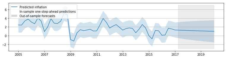
In terms of the reported model diagnostics, this model appears to do a better job of explaining the inflation series - although it is far from perfect.
# Construct the predictions / forecasts
# Notice that now to forecast we need to provide an expanded
# outlier_exog series for the new observations
outlier_exog_fcast = np.zeros((13,1))
inf_forecast3 = inf_results3.get_prediction(
    start='2005-01-01', end='2020-01-01', exog=outlier_exog_fcast)

# Plot them
fig, ax = plt.subplots(figsize=(13, 3), dpi=300)

forecast = inf_forecast3.predicted_mean
ci = inf_forecast3.conf_int(alpha=0.5)

ax.fill_between(forecast.ix['2017-01-02':].index, -10, 7, color='grey',
                alpha=0.15)
lines, = ax.plot(forecast.index, forecast)
ax.fill_between(forecast.index, ci['lower CPIAUCNS'], ci['upper CPIAUCNS'],
                alpha=0.2)

p1 = plt.Rectangle((0, 0), 1, 1, fc="white")
p2 = plt.Rectangle((0, 0), 1, 1, fc="grey", alpha=0.3)
ax.legend([lines, p1, p2], ["Predicted inflation",
                            "In-sample one-step-ahead predictions",
                            "Out-of-sample forecasts"], loc='lower left')
ax.yaxis.grid()