Posterior Simulation
State space models are also amenable to parameter estimation by Bayesian
methods. We consider posterior simulation by Markov chain Monte Carlo (MCMC)
methods, and in particular using the Metropolis-Hastings and Gibbs sampling
algorithms. This section describes how to use the above models in Bayesian
estimation, but fortunately no further modifications need be made; classes
defined as in the maximum likelihood section (i.e. classes that extend from
sm.tsa.statespace.MLEModel) can be used for either maximum
likelihood estimation or Bayesian estimation. Thus the example code here is
only tasked with applying the previously defined state space models.
A full discussion of Bayesian techniques is beyond the scope of this paper, but interested readers can consult [18] for a general introduction to Bayesian econometrics, [34] for a comprehensive Bayesian approach to state space models, and [16] for a excellent practical text on parameter estimation in state space models. The following introduction to Bayesian methods is drawn from these references.
The Bayesian approach to parameter estimation begins by considering parameters as random variables. Bayes’ theorem is applied to derive a distribution for the parameters conditional on the observed data. This “posterior” distribution is proportional to the likelihood function multiplied by a “prior” distribution for the parameters. The prior summarizes all information the researcher has on the parameter values prior to observing the data. Denoting the prior as \(\pi(\psi)\), the likelihood function as \(\mathcal{L}(Y_n \mid \psi)\), and the posterior as \(\pi(\psi \mid Y_n)\), we have
The posterior distribution is the quantity of interest; the difficulty of working with it depends on the prior specified by the researcher and the likelihood function entailed by the selected model. In specific cases (for example the special case of “conjugate priors”) the analytic form of the posterior distribution can be found and used for analysis directly. More often the posterior is not available analytically so other methods must be used to explore its properties.
Posterior simulation is a method available when a procedure exists to sample from the posterior distribution even though the analytic form of the distribution may not be known. Posterior simulation considers drawing samples \(\psi_s, s=1 \dots S\). Under fairly weak conditions a law of large numbers can be applied so that, given the \(S\) samples, sample averages can be used to approximate population quantities
For example, the posterior mean is often of interest and corresponds to \(g(\psi) = \psi\). Histograms can be used to examine the shapes of the marginal distributions of individual parameters.
It may seem that sampling from an unknown distribution is impossible, but MCMC methods allow the eventual sampling from an unknown distribution by applying an algorithm designed to ensure that the unknown distribution is an invariant distribution of a Markov chain. The Markov chain is initialized with an arbitrary value, and then a transition density, denoted \(f(\psi_s \mid \psi_{s-1})\), is applied to draw subsequent values conditional only on the previous value. The appropriate selection of the transition densities can usually ensure that there exists some value \(\hat s\) such that every subsequently drawn sample \(\psi_s, ~ s > \hat s\) is marginally distributed according to the unknown distribution of interest. [1] The two methods discussed below differ in the specification of the transition density.
Markov chain Monte Carlo algorithms
Metropolis-Hastings algorithm [2]
The Metropolis-Hastings algorithm is a very general strategy for constructing a Markov chain with the desired invariant distribution. The transition density is specified in the following way:
Given the current value of the chain, \(\psi_{s-1}\), a proposal value, \(\psi^*\), is selected according to a proposal \(q(\psi ; \psi_{s-1})\) which is a fixed density function for a given value \(\psi_{s-1}\).
With probability \(\alpha(\psi_{s-1}, \psi^*)\) (defined below) the proposed value is accepted so that the next value of the chain is set to \(\psi_s = \psi^*\); if it is not accepted, the chain remains in place \(\psi_s = \psi_{s-1}\).
\[\alpha(\psi_{s-1}, \psi^*) = \min \left \{ \frac{\pi(\psi^* \mid Y_n) q(\psi^* ; \psi_{s-1})}{\pi(\psi_{s-1} \mid Y_n) q(\psi_{s-1} ; \psi^*)}, 1 \right \}\]
Practically speaking, the important component of this algorithm is that only the ratio of posterior quantities is required. Recalling from above that the posterior is proportional to the likelihood and the prior we can rewrite the probability of acceptance as
Given a particular specification for the prior and proposal distributions, this ratio can be computed, where the likelihood function is evaluated as a byproduct of the Kalman filter iterations. In the special case that the proposal distribution satistifes \(q(\psi_{s-1} ; \psi^*) = q(\psi^* ; \psi_{s-1})\) (as will be the case in the examples below), we can again rewrite the probabilty of acceptance as
One convenient choice of proposal distribution that allows this is the so-called random walk proposal with Gaussian increment, defined such that
Notice that to use this proposal distribution, we must set the variance \(\Sigma_\epsilon\). This is often calibrated to achieve some target acceptance rate (ratio of accepted to rejected draws); see the references above for more details.
Gibbs sampling algorithm
Suppose that we can block the parameter vector into \(K\) subvectors, so that \(\psi = \{\psi^{(1)}, \psi^{(2)}, \dots, \psi^{(K)}\}\), and further suppose that all conditional posterior distributions of the form \(\pi(\psi^{(k)} \mid \psi^{(-k)}, Y_n), ~ k=1, \dots, K\) can be sampled from. Then the transition density moving from \(\psi_{s-1}\) to \(\psi_s\) can be defined as follows:
- Given the current value of the chain \(\psi_{s-1}\), sample \(\psi_{s}^{(1)}\) according to the density \(\pi(\psi^{(1)} \mid \psi_{s-1}^{(-1)}, Y_n)\).
- Sample \(\psi_{s}^{(2)}\) according to the density \(\pi(\psi^{(1)} \mid \psi_{s-1}^{(-1,2)}, \psi_{s}^{(1)}, Y_n)\)
- [repeat for \(k=3, \dots, K\)]
- Then \(\psi_s = \{ \psi_s^{(1)}, \psi_s^{(2)}, \dots, \psi_s^{(K)} \}\)
In the case of state space models, we can augment the parameter vector to include the unobserved states. Notice then that the conditional posterior distribution for the states is exactly the distribution from which the simulation smoother produces simulated states; i.e. \(\tilde \alpha\) is drawn according to \(\pi(\alpha \mid \psi, Y_n)\).
The conditional distributions for the parameter vector must be identified on a case-by-case basis. However, notice that the conditional posterior distribution conditions on the unobserved states, so that in many cases the conditional distributions follow from well known econometric problems. For example, if the observation covariance matrix is diagonal, the rows of the observation equation can be viewed as equation-by-equation OLS.
Metropolis-within-Gibbs sampling algorithm
In the case that the parameter vector can be blocked as above but some of the conditional posterior distributions cannot be directly sampled from, a hybrid MCMC approach can be taken. The Gibbs sampling algorithm is used as defined above, except that for any block \(k\) such that the conditional posterior cannot be sampled from, the Metropolis-Hastings algorithm is applied for that block (i.e. a proposal is generated and accepted with the probability defined above).
| [1] | Of course the value \(\hat s\) is unknown and can in some cases be quite large, although statistical tests do exist that can explore this issue. |
| [2] | This discussion is somewhat loose; see [32] and [6] for careful treatments. |
Implementing Metropolis-Hastings: the local level model
In this section we describe implementing the Metropolis-Hastings algorithm to estimate unknown parameters of a state space model. First, it is illuminating to consider a direct approach where all code is explicit. Second, we consider using the another Python library (PyMC) to streamline the estimation process.
The local level, as written above, has two variance parameters
\(\sigma_\varepsilon^2\) and \(\sigma_\eta^2\). In practice we will
sample the standard deviations \(\sigma_\varepsilon\) and
\(\sigma_\eta\). Recalling the Metropolis-Hastings algorithm, in order to
proceed we will need to evaluate the likelihood and the prior and specify a
proposal distribution. The likelihood will be evaluated using the Kalman filter
via the loglike method introduced earlier. The parameters are chosen to
have independent inverse-gamma priors, with the shape and scale parameters set
as in Table 5. [3] We will use the random walk proposal,
which simply requires drawing a value from a multivariate normal distribution
each iteration. We set the variance of the random walk innovation to be the
identity matrix times ten. The prior densities can be evaluated and variates
drawn from the multivariate normal using the Python package SciPy.
| Parameter | Prior distribution | Shape | Scale | Prior mean | Prior variance |
|---|---|---|---|---|---|
| \(\sigma_\varepsilon\) | Inverse-gamma | 3 | 300 | 150 | 22,500 |
| \(\sigma_\eta\) | Inverse-gamma | 3 | 120 | 60 | 3,600 |
For each iteration, the acceptance probability can be calculated from the above elements, and the decision to accept or reject can be made by comparing the acceptance probability to a random variate from a standard uniform distribution.
| [3] | To be clear, since there are multiple ways to parameterize the inverse-gamma distribution, with \(x \sim \text{IG}(\alpha, \beta)\) the density we consider is
\[p(x) = \frac{\beta^\alpha}{\Gamma(\alpha)} x^{-\alpha - 1} e^{-\frac{\beta}{x}}\]
|
Direct approach
Given the existence of the local level class (MLELocalLevel) for
calculating the loglikelihood, the code for performing an MCMC exercise is
relatively simple. First, we initialize the priors and the proposal
distribution
from scipy.stats import multivariate_normal, invgamma, uniform

# Create the model for likelihood evaluation
model = MLELocalLevel(nile)

# Specify priors
prior_obs = invgamma(3, scale=300)
prior_level = invgamma(3, scale=120)

# Specify the random walk proposal
rw_proposal = multivariate_normal(cov=np.eye(2)*10)
Next, we perform 10,000 Metropolis-Hastings iterations as follows. The resultant histograms and traces in terms of the variances, as well as a plot of the acceptance ratio over the iterations, are given in Fig. 11. [4]
# Create storage arrays for the traces
n_iterations = 10000
trace = np.zeros((n_iterations + 1, 2))
trace_accepts = np.zeros(n_iterations)
trace[0] = [120, 30]  # Initial values

# Iterations
for s in range(1, n_iterations + 1):
    proposed = trace[s-1] + rw_proposal.rvs()

    acceptance_probability = np.exp(
        model.loglike(proposed**2) - model.loglike(trace[s-1]**2) +
        prior_obs.logpdf(proposed[0]) + prior_level.logpdf(proposed[1]) -
        prior_obs.logpdf(trace[s-1, 0]) - prior_level.logpdf(trace[s-1, 1]))

    if acceptance_probability > uniform.rvs():
        trace[s] = proposed
        trace_accepts[s-1] = 1
    else:
        trace[s] = trace[s-1]
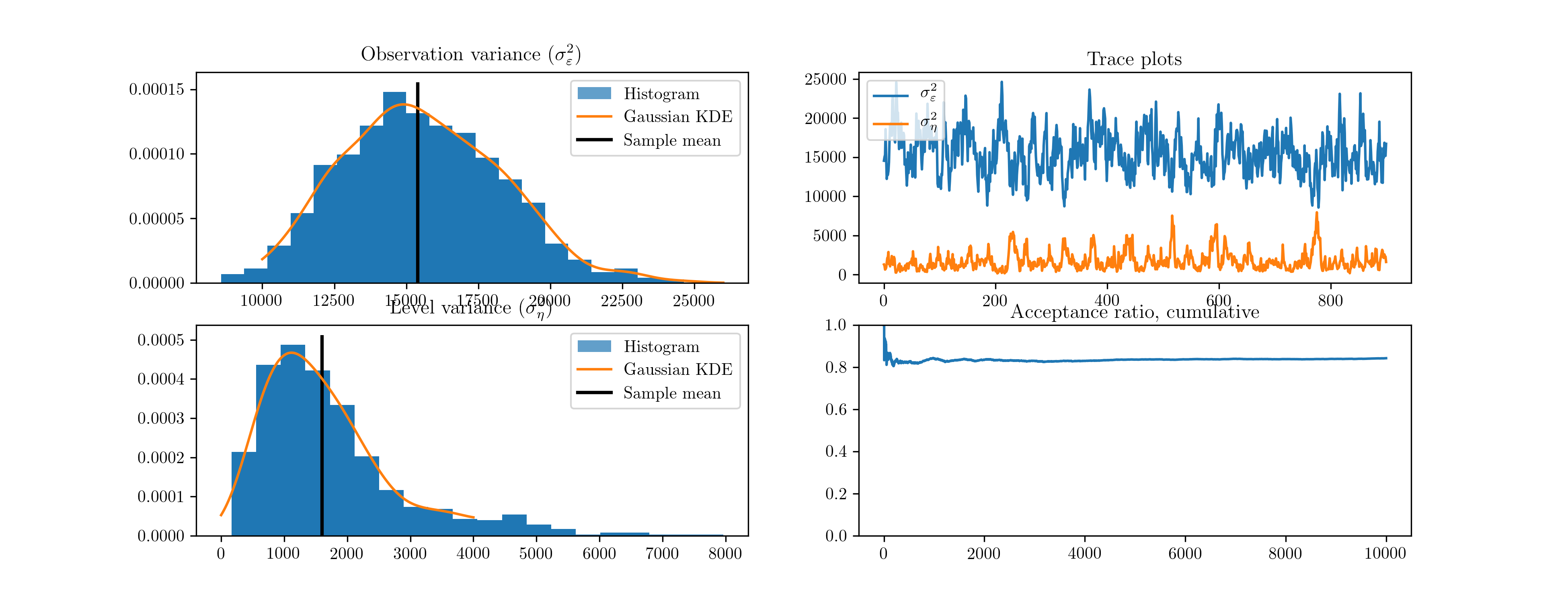
Fig. 11 Output from Metropolis-Hastings posterior simulation on Nile data.
| [4] | The output figures are ultimately based on 900 simulated values for each parameter. Of the 10,000 simulations performed, the first 1,000 were eliminated as the burn-in period and the remaining 9,000 were thinned by only taking each 10th sample, to reduce the effects of autocorrelated draws. |
Integration with PyMC
Parameters can also be simply estimated by taking advantage of the PyMC library ([26]). A full discussion of the features and use of this library is beyond the scope of this paper and instead we only introduce the features we need for estimation of this model. A similar approach would handle most state space models, and the PyMC documentation can be consulted for more advanced usage, including sophisticated sampling techniques such as slice sampling and No-U-Turn sampling.
As above, we need to create objects representing the selected priors and an
object representing the likelihood function. The former are referred to by
PyMC as “stochastic” elements, and the latter as a “data” element (which is
a stochastic element that has already been “observed” and so is not sampled
from). The priors and likelihood function using the MLELocalLevel class
defined above can be implemented with PyMC in the following way
import pymc as mc

# Priors as "stochastic" elements
prior_obs = mc.InverseGamma('obs', 3, 300)
prior_level = mc.InverseGamma('level', 3, 120)

# Create the model for likelihood evaluation
model = MLELocalLevel(nile)

# Create the "data" component (stochastic and observed)
@mc.stochastic(dtype=sm.tsa.statespace.MLEModel, observed=True)
def loglikelihood(value=model, obs_std=prior_obs, level_std=prior_level):
    return value.loglike([obs_std**2, level_std**2])
We do not need to explicitly specify the proposal; PyMC uses an adaptive proposal by default. Instead, we simply need to create a “model”, which unifies the priors and likelihood, and a “sampler”. The sampler is an object used to perform the simulations and return the trace objects. The resultant histograms and traces in terms of the variances from 10,000 iterations are given in Fig. 12. [5]
# Create the PyMC model
pymc_model = mc.Model((prior_obs, prior_level, loglikelihood))

# Create a PyMC sample and perform sampling
sampler = mc.MCMC(pymc_model)
sampler.sample(iter=10000, burn=1000, thin=10)
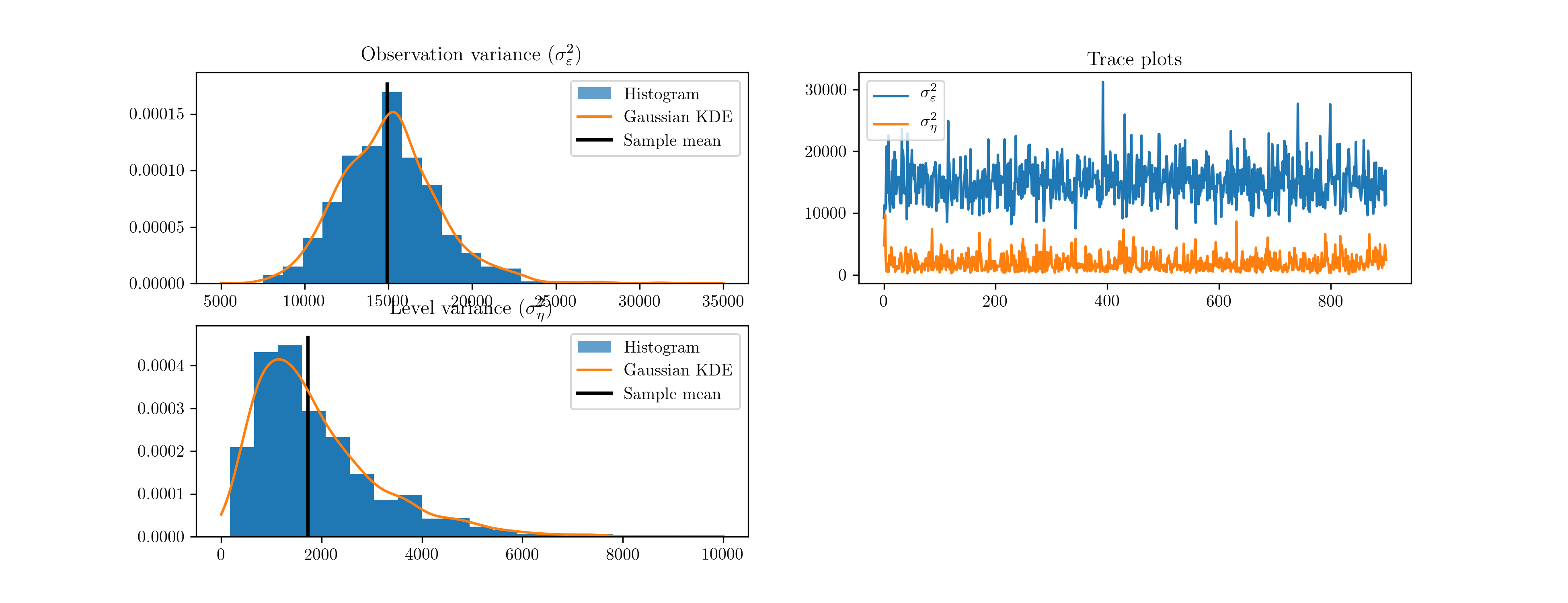
Fig. 12 Output from Metropolis-Hastings posterior simulation on Nile data, using the PyMC library.
| [5] | The acceptance ratio is not provided by PyMC when the adaptive proposal is used. |
Implementing Gibbs sampling: the ARMA(1,1) model
In this section we describe implementing the Gibbs sampling algorithm to estimation unknown parameters of a state space model. Only the direct approach is presented here (as of now, PyMC only has preliminary support for Gibbs sampling). The Metropolis-within-Gibbs approach is used to demonstrate both how to apply Gibbs sampling and how to apply a hybrid approach.
Recalling the Gibbs sampling algorithm, in order to proceed we need to block the parameters and the unobserved states such the the conditional distributions can be found. We will choose four blocks, so that the unobserved states are in the first block, the autoregressive coefficient is in the second block, the variance is in the third block, and the moving average coefficient is in the last block. In notation, this means that \(\psi = \{ \psi^{(1)}, \psi^{(2)}, \psi^{(3)}, \psi^{(4)} \} = \{ \alpha, \phi, \sigma^2, \theta \}\). We will apply Gibbs steps for the first, second, and third blocks and a Metropolis step for the fourth block.
We select priors for the parameters so that the conditional posterior distributions that we require can be constructed. For the autogressive coefficients we select a multivariate normal distribution - conditional on the variance - with an identity covariance matrix and restricted to the space such that the corresponding lag polynomial is invertible. To be precise, the prior is \(\phi \mid \sigma^2 \sim N(0, I)\) such that \(\phi(L)\) is invertible.
For the variance, we select an inverse-gamma distribution - conditional on the autoregressive coefficients - with the shape and scale parameters both set to three. To be precise, the prior is \(\sigma^2 \mid \phi \sim IG(3, 3)\). These choices will be convenient due to their status as conjugate priors for the linear regression model; they will lead to known conditional posterior distributions.
Finally, the prior for the moving-average coefficient is specified to be uniform over the interval \((-1, 1)\), so that \(\theta \sim \text{unif}(-1, 1)\). Notice that the prior density for all values in the range is equal, and so the acceptance probability is either zero, in the case that the proposed value is outside the range, or else simplifies to the ratio of the likelihoods because the prior values cancel out. We will use a random walk proposal with standard Gaussian increment.
Now, conditional on the model parameters, a draw of \(\psi^{(1)}\) can be taken by applying the simulation smoother as shown in previous sections. Next notice that, given the values of the states, the first row of the transition equation in (?) is simply a linear regression:
Stacking these equations across all \(t\) into matrix form yields \(Z = X \phi + \varepsilon\). A standard result applying conjugate priors to the linear regression model (see for example [16]) is that the conditional posterior distribution for the coefficients is Gaussian and the conditional posterior distribution for the variance is inverse-gamma. To be precise, given our choice of prior hyperparameters here we have
Making draws from these conditional posteriors can be implemented in the following way
from scipy.stats import multivariate_normal, invgamma

def draw_posterior_phi(model, states, sigma2):
    Z = states[0:1, 1:]
    X = states[0:1, :-1]

    tmp = np.linalg.inv(sigma2 * np.eye(1) + np.dot(X, X.T))
    post_mean = np.dot(tmp, np.dot(X, Z.T))
    post_var = tmp * sigma2

    return multivariate_normal(post_mean, post_var).rvs()

def draw_posterior_sigma2(model, states, phi):
    resid = states[0, 1:] - phi * states[0, :-1]
    post_shape = 3 + model.nobs
    post_scale = 3 + np.sum(resid**2)

    return invgamma(post_shape, scale=post_scale).rvs()
Implementing the hybrid method then consists of the following steps for each iteration, given the previous value \(\psi_{s-1}\).
- Apply the simulation smoother to retrieve a draw of the unobserved states, yielding \(\tilde \alpha = \psi_s^{(1)}\).
- Draw a value for \(\phi = \psi_1^{(2)}\) from its conditional posterior distribution, conditioning on the states drawn in step 1 and the parameters from the previous iteration.
- Draw a value for \(\sigma^2 = \psi_s^{(3)}\) from its conditional posterior distribution, conditioning on the state states drawn in step 1 and the autoregression coefficients drawn in step 2.
- Propose a new value for \(\theta = \psi_s^{(4)}\) using the random walk
proposal, and calculate the acceptance probability using the
loglikefunction.
The implementation code is below, and the resultant histograms and traces from 10,000 iterations are given in Fig. 13.
from scipy.stats import norm, uniform
from statsmodels.tsa.statespace.tools import is_invertible

# Create the model for likelihood evaluation and the simulation smoother
model = ARMA11(inf)
sim_smoother = model.simulation_smoother()

# Create the random walk and comparison random variables
rw_proposal = norm(scale=0.3)

# Create storage arrays for the traces
n_iterations = 10000
trace = np.zeros((n_iterations + 1, 3))
trace_accepts = np.zeros(n_iterations)
trace[0] = [0, 0, 1.]  # Initial values

# Iterations
for s in range(1, n_iterations + 1):
    # 1. Gibbs step: draw the states using the simulation smoother
    model.update(trace[s-1], transformed=True)
    sim_smoother.simulate()
    states = sim_smoother.simulated_state[:, :-1]

    # 2. Gibbs step: draw the autoregressive parameters, and apply
    # rejection sampling to ensure an invertible lag polynomial
    phi = draw_posterior_phi(model, states, trace[s-1, 2])
    while not is_invertible([1, -phi]):
        phi = draw_posterior_phi(model, states, trace[s-1, 2])
    trace[s, 0] = phi

    # 3. Gibbs step: draw the variance parameter
    sigma2 = draw_posterior_sigma2(model, states, phi)
    trace[s, 2] = sigma2

    # 4. Metropolis-step for the moving-average parameter
    theta = trace[s-1, 1]
    proposal = theta + rw_proposal.rvs()
    if proposal > -1 and proposal < 1:
        acceptance_probability = np.exp(
            model.loglike([phi, proposal, sigma2]) -
            model.loglike([phi, theta, sigma2]))

        if acceptance_probability > uniform.rvs():
            theta = proposal
            trace_accepts[s-1] = 1
    trace[s, 1] = theta
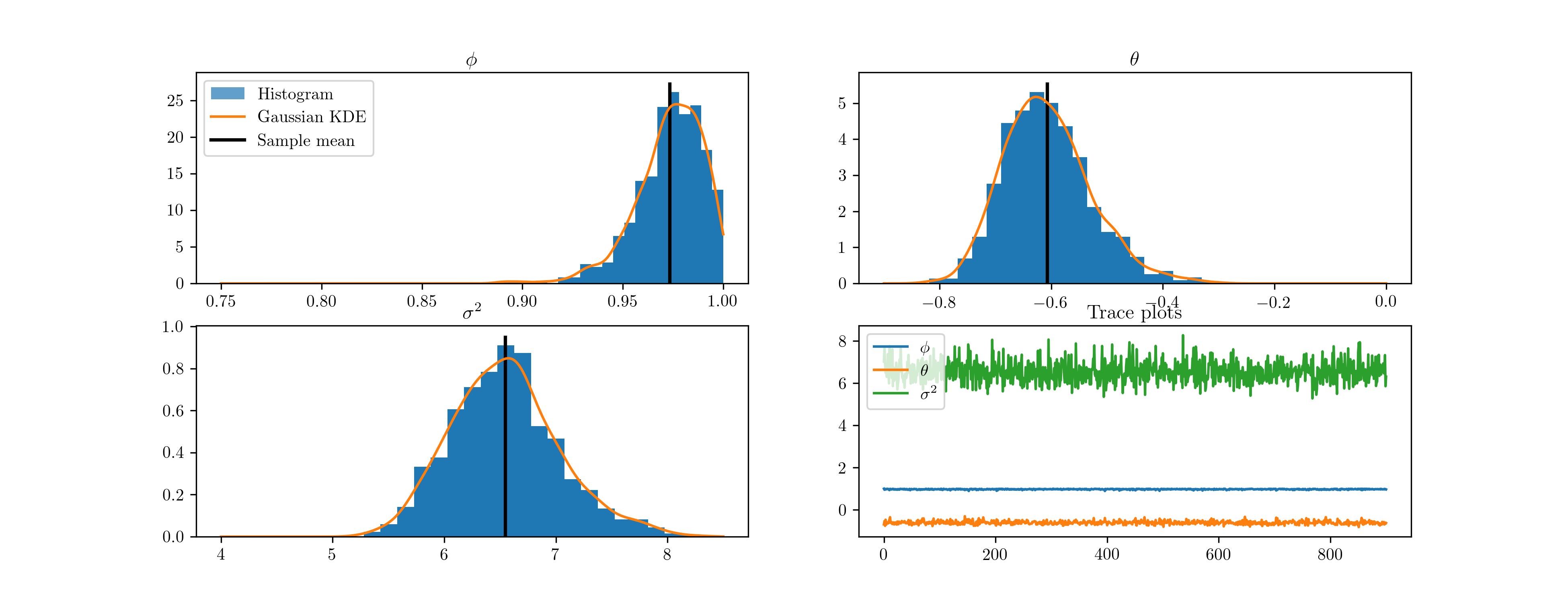
Fig. 13 Output from Metropolis-within-Gibbs posterior simulation on US CPI inflation data.
Implementing Gibbs sampling: real business cycle model
Finally, we can apply the same techniques as above to perform Metropolis-within-Gibbs estimation of the real business cycle model parameters. It is often difficult to estimate all of the parameters of the RBC model, or other structural models, by maximum likelihood. Indeed, above we only estimated two of the six structural parameters. By choosing appropriately tight priors it is often feasible to estimate more parameters; in this example we estimate four of the six structural parameters: the discount rate, capital share, and the two technology shock parameters. Of the two remaining parameters, the disutility of labor only serves to pin down steady-state values and so the model presented above is independent of its value (since it considers data in in deviation-from-steady-state values), and the depreciation rate is best calibrated when the observation datasets do not speak to to depreciation (see, for example, the discussion in [30]).
For the Metropolis-within-Gibbs simulation, we consider 8 blocks. The first three blocks are sampled using Gibbs steps, and are very similar to the ARMA(1,1) example; the first block samples the unobserved states, and the second and third blocks sample the two technology shock parameters. Noticing that the second row of the transition equation is simply an autoregression, conditional on the states, we can use the same approach as before. Thus the priors on these parameters are the Gaussian and inverse-gamma conjugate priors and the unobserved states are sampled using the simulation smoother.
The remaining blocks apply Metropolis steps to sample the remaining five parameters: the discount rate, capital share, and the three measurement variances. The priors on these parameters are as in [30]. All priors are listed in Table 6, along with statistics describing the posterior draws.
| Prior distribution | Posterior distribution | ||||||
|---|---|---|---|---|---|---|---|
| Distribution | Mean | Std. Dev. | Mode | Mean | 5 percent | 95 percent | |
| Discount rate [6] | Gamma | 0.25 | 0.1 | 0.997 | 0.997 | 0.994 | 0.998 |
| Capital share | Normal | 0.3 | 0.01 | 0.325 | 0.325 | 0.308 | 0.341 |
| Technology shock persistence | Normal | 0 | 1 | 0.672 | 0.637 | -0.271 | 0.940 |
| Technology shock variance | Inverse-gamma | 0.01 | 1.414 | 8.65e-5 | 8.98e-5 | 7.67e-5 | 1.05e-4 |
| Output error standard deviation | Inverse-gamma | 0.1 | 2 | 2.02e-5 | 2.29e-5 | 1.46e-5 | 3.34e-05 |
| Labor error standard deviation | Inverse-gamma | 0.1 | 2 | 3.06e-5 | 3.21e-5 | 2.25e-5 | 4.34e-05 |
| Consumption error standard deviation | Inverse-gamma | 0.1 | 2 | 2.46e-5 | 2.57e-5 | 1.94e-5 | 3.28e-05 |
Again, the code is slightly too long to display inline, so it can be found in Appendix C: Real business cycle model code. We perform 100,000 draws and burn the first 10,000. Of the remaining 90,000 draws, each tenth draw is saved, so that the results below are ultimately based on 9,000 draws. Histograms of the four estimated structural parameters are presented in Fig. 14.
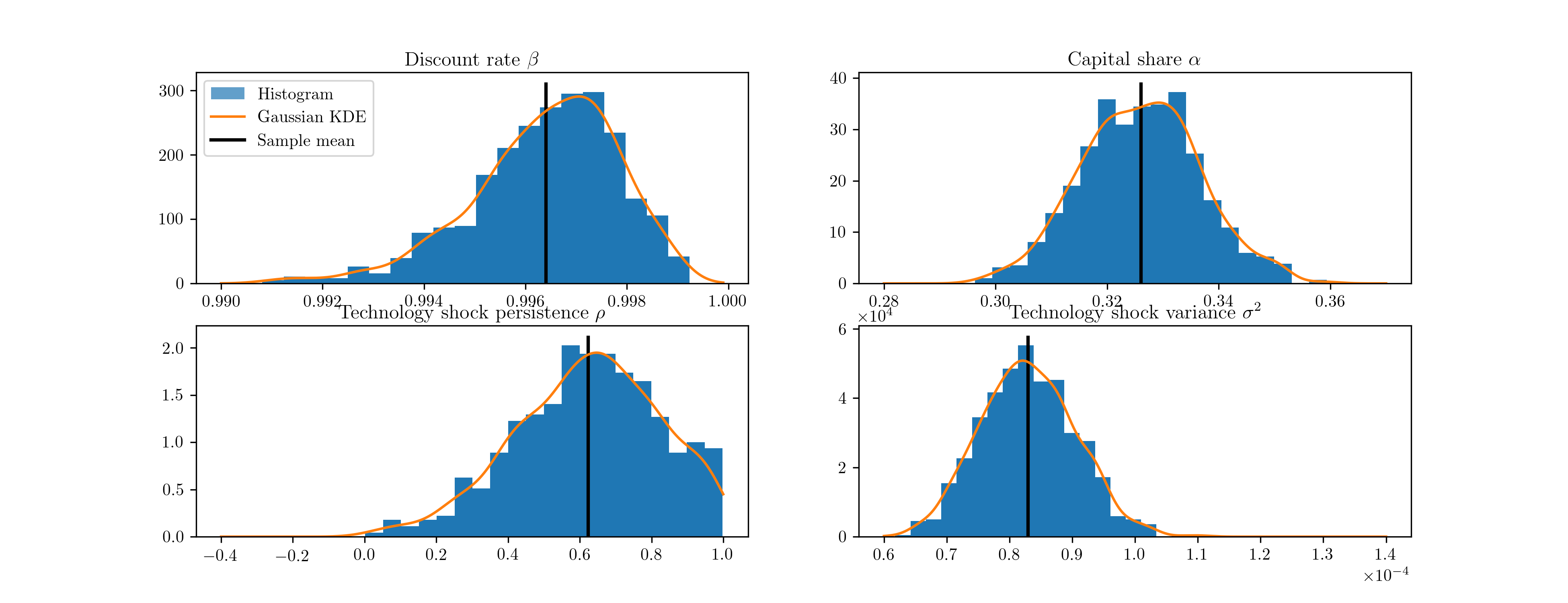
Fig. 14 Output from Metropolis-within-Gibbs posterior simulation of the real business cycle.
As before, we may be interested in the implied impulse response functions and the smoothed state values; here we calculate these by applying the Kalman filter and smoother to the model based on the median parameter values. Fig. 15 displays the impulse responses and Fig. 16 displays the smoothed states and confidence intervals.
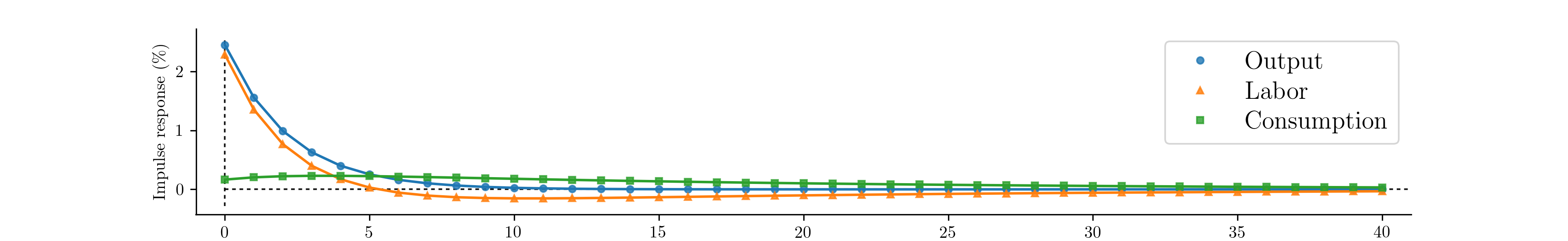
Fig. 15 Impulse response functions corresponding to Metropolis-within-Gibbs estimation of the real business cycle.
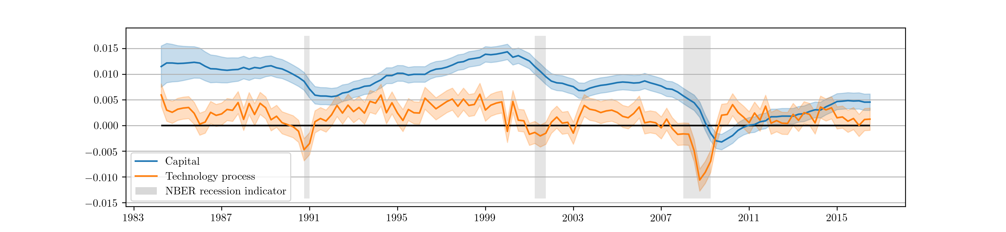
Fig. 16 Smoothed estimates of capital and the technology process from Metropolis-within-Gibbs estimation of the real business cycle.
| [6] | If the discount rate is denoted \(\beta\), then the Gamma prior actually applies to the transformation \(100 (\beta^{-1} - 1)\). |