Out-of-the-box models
This paper has focused on demonstrating the creation of classes to specify
and estimate arbitrary state space models. However, it is worth noting that
classes implementing state space models for four of the most popular models in
time series analysis are built in. These classes have been created
exactly as described above (e.g. they are all subclasses of
sm.tsa.statespace.MLEModel), and can be used directly or even extended with
their own subclasses. The source code is available, so that they also serve as
advanced examples of what can be accomplished in this framework.
Maximum likelihood estimation is available immediately simply by calling the
fit method. Features include the calculation of reasonable starting values,
the use of appropriate parameter transformations, and enhanced results classes.
Bayesian estimation via posterior simulation can be performed as described
in this paper by taking advantage of the loglike method and the simulation
smoother. Of course the selection of priors, parameter blocking, etc. must be
manually implemented, as above.
In this section, we briefly describe each time series model and provide examples.
SARIMAX
The seasonal autoregressive integrated moving-average with exogenous regressors (SARIMAX) model is a generalization of the familiar ARIMA model to allow for seasonal effects and explanatory variables. It is typically denoted SARIMAX \((p,d,q)\times(P,D,Q,s)\) and can be written as
where \(y_t\) is the observed time series and \(x_t\) are explanatory regressors. \(\phi_p(L), \tilde \phi_P(L^s), \theta_q(L),\) and \(\tilde \theta_Q(L^s)\) are lag polynomials and \(\Delta^d\) is the differencing operator \(\Delta\), applied \(d\) times. This model is sometimes described as regression with SARIMA errors.
It is straightforward to apply this model to data by creating an instance of
the class sm.tsa.SARIMAX. For example, if we wanted to estimate an
ARMA(1,1) model for US CPI inflation data using this class, the following
code could be used
model_1 = sm.tsa.SARIMAX(inf, order=(1, 0, 1))
results_1 = model_1.fit()
print(model_1.loglike(results_1.params))  # -432.375194381
We can also extend this example to take into account annual seasonality. Below we estimate an SARIMA(1,0,1)x(1,0,1,12) model. This model achieves a lower value for the Akaike information criterion (AIC), which indicates a potentially better fit. [1]
model_2 = sm.tsa.SARIMAX(inf, order=(1, 0, 1), seasonal_order=(1, 0, 1, 12))
results_2 = model_2.fit()

# Compare the two models on the basis of the Akaike information criterion
print(results_1.aic)  # 870.750388763
print(results_2.aic)  # 844.623363003
| [1] | The Akaike information criterion, as well as several other information
criteria, is available for all models that extend the
sm.tsa.statespace.MLEModel class. See the tables in
Appendix B: Inherited attributes and methods for all available attributes and methods. |
Unobserved components
Unobserved components models, also known as structural time series models, decompose a univariate time series into trend, seasonal, cyclical, and irregular components. They can be written as:
where \(y_t\) refers to the observation vector at time \(t\),
\(\mu_t\) refers to the trend component, \(\gamma_t\) refers to the
seasonal component, \(c_t\) refers to the cycle, and
\(\varepsilon_t\) is the irregular. The modeling details of these
components can be found in the package documentation. These models are also
described in depth in Chapter 3 of [10]. The class
corresponding to these models is sm.tsa.UnobservedComponents.
As an example, consider extending the model previously applied to the Nile river data to include a stochastic cycle, as suggested in [23]. This is straightforward with the built-in model; the below example fits the model and plots the unobserved components, in this case a level and a cycle, in Fig. 17.
model = sm.tsa.UnobservedComponents(nile, 'llevel', cycle=True, stochastic_cycle=True)
results = model.fit()
fig = results.plot_components(observed=False)
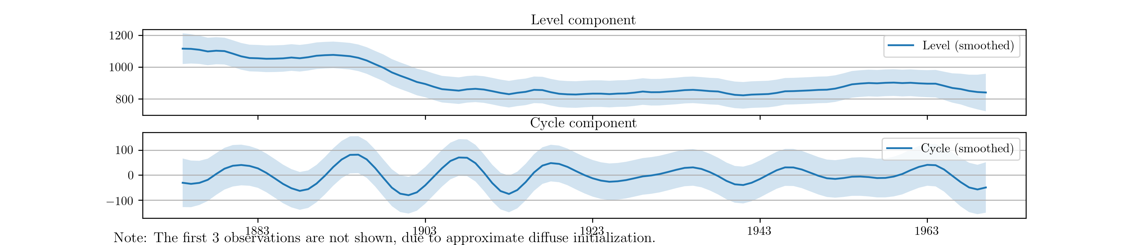
Fig. 17 Estimates of the unobserved level and cyclical components of Nile river volume.
VAR
Vector autoregressions are important tools for reduced form time series analysis of multiple variables. Their form looks similar to an AR(p) model except that the variables are vectors and the coefficients are matrices.
These models can be estimated using the sm.tsa.VARMAX class, which also
allows estimation of vector moving average models and optionally models with
exogenous regressors. [2] The following code estimates a vector autoregression
as a state space model (the starting parameters are the OLS estimates) and
generates orthogonalized impulse response functions for shocks to each of the
endogenous variables; these responses are plotted in
Fig. 18. [3]
model = sm.tsa.VARMAX(rbc_data, order=(1, 0))
results = model.fit()

# Generate impulse response functions; the `impluse` argument is used to
# specify which shock is pulsed.
output_irfs = results.impulse_responses(15, impulse=0, orthogonalized=True) * 100
labor_irfs = results.impulse_responses(15, impulse=1, orthogonalized=True) * 100
consumption_irfs = results.impulse_responses(15, impulse=2, orthogonalized=True) * 100
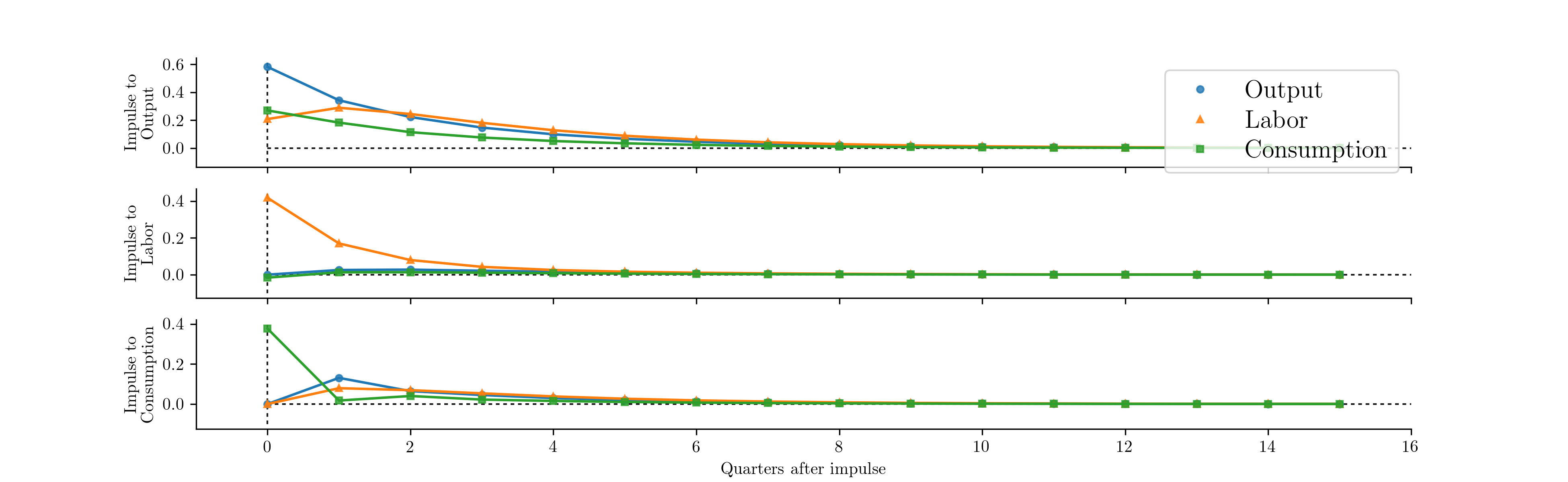
Fig. 18 Impulse response functions derived from a vector autoregression.
| [2] | Estimation of VARMA(p,q) models is practically possible, although it is not recommended because no measures are in place to ensure identification (for example, the use of Kronecker indices is not yet available). |
| [3] | Note that the orthogonalization is by Cholesky decomposition, which
implicitly enforces a a causal ordering to the variables. The order is
as defined in the provided dataset. Here rbc_data orders the
variables as output, labor, consumption. |
Dynamic factors
Dynamic factor models are another set of important reduced form multivariate models. They can be used to extract a common component from multifarious data. The general form of the model available here is the so-called static form of the dynamic factor model and can be written
where \(y_t\) is the endogenous data, \(f_t\) are the unobserved factors which follow a vector autoregression, and \(x_t\) are optional exogenous regressors. \(\eta_t\) and \(\varepsilon_t\) are white noise error terms, and \(u_t\) allows the possibility of autoregressive (or vector autoregressive) errors. In order to identify the factors, \(Var(\eta_t) \equiv I\).
The following code extracts a single factor that follows an AR(2) process. The error term is not assumed to be autoregressive, so in this case \(u_t = \varepsilon_t\). By default the model assumes the elements of \(\varepsilon_t\) are not cross-sectionally correlated (this assumption can be relaxed if desired). Fig. 19 plots the responses of the endogenous variables to an impulse in the unobserved factor.
model = sm.tsa.DynamicFactor(rbc_data, k_factors=1, factor_order=2)
results = model.fit()
print(results.coefficients_of_determination)  # [ 0.957   0.545   0.603 ]

# Because the estimated factor turned out to be inversely related to the
# three variables, we want to consider the negative of the impulse
dfm_irfs = -results.impulse_responses(15, impulse=0, orthogonalized=True) * 100
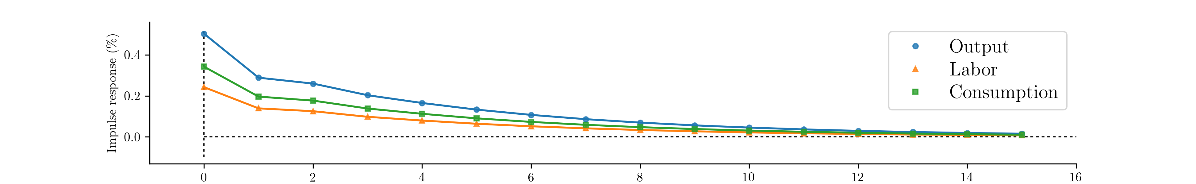
Fig. 19 Impulse response functions derived from a dynamic factor model.
It is often difficult to directly interpret either the filtered estimates of
the unobserved factors or the estimated coefficients of the \(\Lambda\)
matrix (called the matrix of factor loadings) due to identification issues
related to the factors. For example, notice that
\(\Lambda f_t = (-\Lambda) (-f_t)\) so that reversing the signs of the
factors and loadings results in an identical model. It is often
informative instead to examine the extent to which each unobserved factor
explains each endogenous variable (see for example
[14]). This can be explored using the
\(R^2\) value from the regression of each endogenous variable on each
estimated factor and a constant. These values are available in the results
attribute coefficients_of_determination. For the model estimated above, it
is clear that the estimated factor largely tracks output.