Maximum Likelihood Estimation
Classical estimation of parameters in state space models is possible because
the likelihood is a byproduct of the filtering recursions. Given a set of
initial parameters, numerical maximization techniques, often quasi-Newton
methods, can be applied to find the set of parameters that maximize (locally)
the likelihood function, \(\mathcal{L}(Y_n \mid \psi)\). In this section we
describe how to apply maximum likelihood estimation (MLE) to state space models
in Python. First we show how to apply a minimization algorithm in SciPy to
maximize the likelihood, using the loglike method. Second, we show how the underlying Statsmodels functionality inherited by our subclasses can be used to
greatly streamline estimation.
In particular, models extending from the sm.tsa.statespace.MLEModel
(“MLEModel”) class can painlessly perform maximum likelihood estimation via
a fit method. In addition, summary tables, postestimation results, and
model diagnostics are available. Appendix B: Inherited attributes and methods describes all of the
methods and attributes that are available to subclasses of MLEModel
and to results objects.
Direct approach
Numerical optimziation routines in Python are available through the Python package SciPy ([13]). Generically, these are in the form of minimizers that accept a function and a set of starting parameters and return the set of parameters that (locally) minimize the function. There are a number of available algorithms, including the popular BFGS (Broyden–Fletcher–Goldfarb–Shannon) method. As is usual when minimization routines are available, in order to maximize the (log) likelihood, we minimize its negative.
The code below demonstrates how to apply maximum likelihood estimation to the
LocalLevel class defined in the previous section for the Nile dataset. In
this case, because we have not bothered to define good starting parameters, we
use the Nelder-Mead algorithm that can be more robust than BFGS although it
may converge more slowly.
# Load the generic minimization function from scipy
from scipy.optimize import minimize

# Create a new function to return the negative of the loglikelihood
nile_model_2 = LocalLevel(nile)
def neg_loglike(params):
    return -nile_model_2.loglike(params)

# Perform numerical optimization
output = minimize(neg_loglike, nile_model_2.start_params, method='Nelder-Mead')

print(output.x)  # [ 15108.31   1463.55]
print(nile_model_2.loglike(output.x))  # -632.537685587
The maximizing parameters are very close to those reported by [10] and achieve a negligibly higher loglikelihood (-632.53769 versus -632.53770).
Integration with Statsmodels
While likelihood maximization itself can be performed relatively easily, in practice there are often many other desired quantities aside from just the optimal parameters. For example, inference often requires measures of parameter uncertainty (standard errors and confidence intervals). Another issue that arises is that it is most convenient to allow the numerical optimizer to choose parameters across the entire real line. This means that some combinations of parameters chosen by the optimizer may lead to an invalid model specification. It is sometimes possible to use an optimization procedure with constraints or bounds, but it is almost always easier to allow the optimizer to choose in an unconstrained way and then to transform the parameters to fit the model. The implementation of parameter transformations will be discussed at greater length below.
While there is no barrier to users calculating those quantities or implementing
transformations, the calculations are standard and there is no reason for each
user to implement them separately. Again we turn to the principle of separation
of concerns made possible through the object oriented programming approach,
this time by making use of the tools available in Statsmodels. In particular, a
new method, fit, is available to automatically perform maximum
likelihood estimation using the starting parameters defined in the
start_params attribute (see above) and returns a results object.
The following code further refines the local level model by adding a new
attribute param_names that augments output with descriptive parameter
names. There is also a new line in the update method that implements
parameter transformations: the params vector is replaced with the output
from the update method of the parent class (MLEModel). If the
parameters are not already transformed, the parent update method calls the
appropriate transformation functions and returns the transformed parameters. In
this class we have not yet defined any transformation functions, so the parent
update method will simply return the parameters it was given. Later we will
improve the class to force the variance parameter to be positive.
class FirstMLELocalLevel(sm.tsa.statespace.MLEModel):
    start_params = [1.0, 1.0]
    param_names = ['obs.var', 'level.var']

    def __init__(self, endog):
        super(FirstMLELocalLevel, self).__init__(endog, k_states=1)

        self['design', 0, 0] = 1.0
        self['transition', 0, 0] = 1.0
        self['selection', 0, 0] = 1.0

        self.initialize_approximate_diffuse()
        self.loglikelihood_burn = 1

    def update(self, params, **kwargs):
        # Transform the parameters if they are not yet transformed
        params = super(FirstMLELocalLevel, self).update(params, **kwargs)

        self['obs_cov', 0, 0] = params[0]
        self['state_cov', 0, 0] = params[1]
With this new definition, we can instantiate our model and perform maximum
likelihood estimation. As one feature of the integration with Statsmodels, the
result object has a summary method that prints a table of results:
nile_mlemodel_1 = FirstMLELocalLevel(nile)

print(nile_mlemodel_1.loglike([15099.0, 1469.1]))  # -632.537695048

# Again we use Nelder-Mead; now specified as method='nm'
nile_mleresults_1 = nile_mlemodel_1.fit(method='nm', maxiter=1000)
print(nile_mleresults_1.summary())
                           Statespace Model Results
==============================================================================
Dep. Variable:                 volume   No. Observations:                  100
Model:             FirstMLELocalLevel   Log Likelihood                -632.538
Date:                Sat, 28 Jan 2017   AIC                           1269.075
Time:                        15:19:50   BIC                           1274.286
Sample:                    01-01-1871   HQIC                          1271.184
                         - 01-01-1970
Covariance Type:                  opg
==============================================================================
                 coef    std err          z      P>|z|      [0.025      0.975]
------------------------------------------------------------------------------
obs.var     1.511e+04   2586.966      5.840      0.000       1e+04    2.02e+04
level.var   1463.5472    843.717      1.735      0.083    -190.109    3117.203
===================================================================================
Ljung-Box (Q):                       36.00   Jarque-Bera (JB):                 0.05
Prob(Q):                              0.65   Prob(JB):                         0.98
Heteroskedasticity (H):               0.61   Skew:                            -0.03
Prob(H) (two-sided):                  0.16   Kurtosis:                         3.08
===================================================================================

Warnings:
[1] Covariance matrix calculated using the outer product of gradients (complex-step).
A second feature is the availability of model diagnostics. Test statistics for
tests of the standardized residuals for normality, heteroskedasticity, and
serial correlation are reported at the bottom of the summary output. Diagnostic
plots can also be produced using the plot_diagnostics method, illustrated
in Fig. 6. [1] Notice that Statsmodels is aware of the
date index of the Nile dataset and uses that information in the summary table
and diagnostic plots.
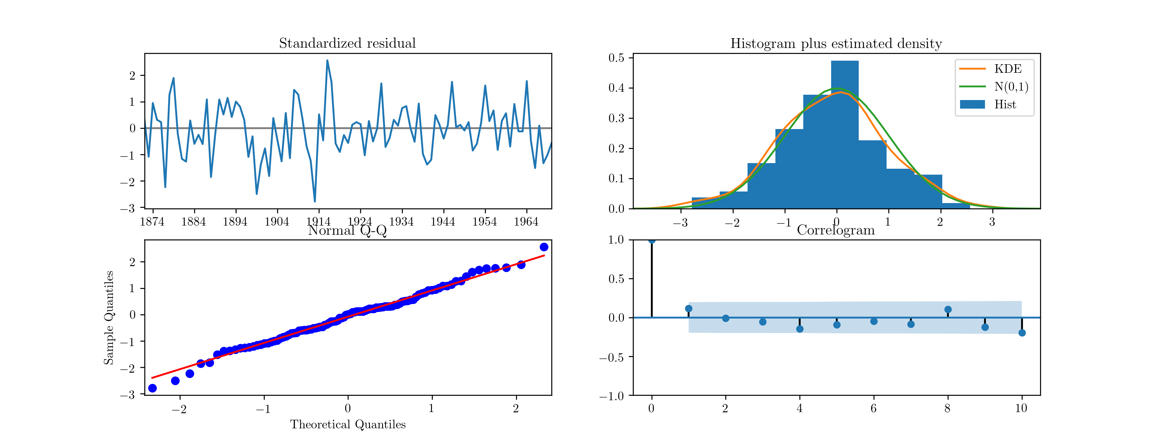
Fig. 6 Diagnostic plots for standardised residuals after maximum likelihood estimation on Nile data.
A third feature is the availability of forecasting (through the
get_forecasts method) and impulse response functions (through the
impulse_responses method). Due to the nature of the local level model these
are uninteresting here, but will be exhibited in the ARMA(1,1) and real
business cycle examples below.
| [1] | See sections 2.12 and 7.5 of [10] for a description of the standardized residuals and the definitions of the provided diagnostic tests. |
Parameter transformations
As mentioned above, parameter transformations are an important component of maximum likelihood estimation in a wide variety of cases. For example, in the local level model above the two estimated parameters are variances, which cannot theoretically be negative. Although the optimizer avoided the problematic regions in the above example, that will not always be the case. As another example, ARMA models are typically assumed to be stationary. This requires coefficients that permit inversion of the associated lag polynomial. Parameter transformations can be used to enforce these and other restrictions.
For example, if an unconstrained variance parameter is squared the transformed variance parameter will always be positive. [24] and [2] describe transformations sufficient to induce stationarity in the univariate and multivariate cases, respectively, by taking advantage of the one-to-one correspondence between lag polynomial coefficients and partial autocorrelations. [2]
It is strongly preferred that the transformation function have a well-defined inverse so that starting parameters can be specified in terms of the model space and then “untransformed” to appropriate values in the unconstrained space.
Implementing parameter transformations when using MLEModel as the base
class is as simple as adding two new methods: transform_params and
untransform_params (if no parameter transformations as required, these
methods can simply be omitted from the class definition). The following code
redefines the local level model again, this time to include parameter
transformations to ensure positive variance parameters. [3]
class MLELocalLevel(sm.tsa.statespace.MLEModel):
    start_params = [1.0, 1.0]
    param_names = ['obs.var', 'level.var']

    def __init__(self, endog):
        super(MLELocalLevel, self).__init__(endog, k_states=1)

        self['design', 0, 0] = 1.0
        self['transition', 0, 0] = 1.0
        self['selection', 0, 0] = 1.0

        self.initialize_approximate_diffuse()
        self.loglikelihood_burn = 1

    def transform_params(self, params):
        return params**2

    def untransform_params(self, params):
        return params**0.5

    def update(self, params, **kwargs):
        # Transform the parameters if they are not yet transformed
        params = super(MLELocalLevel, self).update(params, **kwargs)

        self['obs_cov', 0, 0] = params[0]
        self['state_cov', 0, 0] = params[1]
All of the code given above then applies equally to this new model, except that this class is robust to the optimizer selecting negative parameters.
| [2] | The transformations to induce stationarity are made available in this
package as the functions
sm.tsa.statespace.tools.constrain_stationary_univariate and
sm.tsa.statespace.tools.constrain_stationary_multivariate. Their
inverses are also available. |
| [3] | Note that in Python, the exponentiation operator is **. |
Example models
In this section, we extend the code from Representation in Python to allow for maximum likelihood estimation through Statsmodels integration.
ARMA(1, 1) model
from statsmodels.tsa.statespace.tools import (constrain_stationary_univariate,
                                              unconstrain_stationary_univariate)

class ARMA11(sm.tsa.statespace.MLEModel):
    start_params = [0, 0, 1]
    param_names = ['phi', 'theta', 'sigma2']

    def __init__(self, endog):
        super(ARMA11, self).__init__(
            endog, k_states=2, k_posdef=1, initialization='stationary')

        self['design', 0, 0] = 1.
        self['transition', 1, 0] = 1.
        self['selection', 0, 0] = 1.

    def transform_params(self, params):
        phi = constrain_stationary_univariate(params[0:1])
        theta = constrain_stationary_univariate(params[1:2])
        sigma2 = params[2]**2
        return np.r_[phi, theta, sigma2]

    def untransform_params(self, params):
        phi = unconstrain_stationary_univariate(params[0:1])
        theta = unconstrain_stationary_univariate(params[1:2])
        sigma2 = params[2]**0.5
        return np.r_[phi, theta, sigma2]

    def update(self, params, **kwargs):
        # Transform the parameters if they are not yet transformed
        params = super(ARMA11, self).update(params, **kwargs)

        self['design', 0, 1] = params[1]
        self['transition', 0, 0] = params[0]
        self['state_cov', 0, 0] = params[2]
The parameters can now be easily estimated via maximum likelihood using the
fit method. This model also allows us to demonstrate the prediction and
forecasting features provided by the Statsmodels integration. In particular, we
use the get_prediction method to retrieve a prediction object that gives
in-sample one-step-ahead predictions and out-of-sample forecasts, as well as
confidence intervals. Fig. 7 shows a graph of the
output.
inf_model = ARMA11(inf)
inf_results = inf_model.fit()

inf_forecast = inf_results.get_prediction(start='2005-01-01', end='2020-01-01')
print(inf_forecast.predicted_mean)  # [2005-01-01   2.439005 ...
print(inf_forecast.conf_int())      # [2005-01-01   -2.573556 7.451566 ...
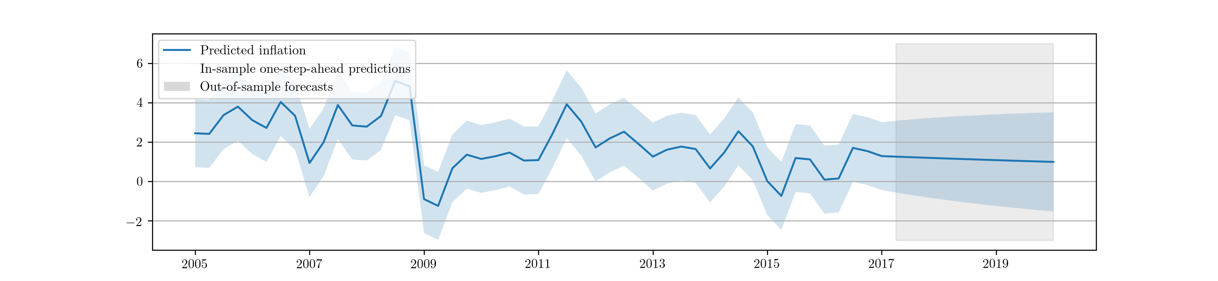
Fig. 7 In-sample one-step-ahead predictions and out-of-sample forecasts for ARMA(1,1) model on US CPI inflation data.
If only out-of-sample forecasts had been desired, the get_forecasts
method could have been used instead, and if only the forecasted values had
been desired (and not additional results like confidence intervals), the
methods predict or forecast could have been used.
Local level model
See the previous sections for the Python implementation of the local level model.
Real business cycle model
Due to the the complexity of the model, the full code for the model is too
long to display inline, but it is provided in the Appendix C: Real business cycle model code. It
implements the real business cycle model in a class named SimpleRBC and
allows selecting some of the structural parameters to be estimated while
allowing others to be calibrated (set to specific values).
Often in structural models one of the outcomes of interest is the time paths of the observed variables following a hypothetical structural shock; these time paths are called impulse response functions, and they can be generated for any state space model.
In the first application, we will calibrate all of the structural parameters to
the values suggested in [27] and simply estimate
the measurement error variances (these do not affect the model dynamics or the
impulse responses). Once the model has been estimated, the
impulse_responses method can be used to generate the time paths.
# Calibrate everything except measurement variances
calibrated = {
    'discount_rate': 0.95,
    'disutility_labor': 3.0,
    'capital_share': 0.36,
    'depreciation_rate': 0.025,
    'technology_shock_persistence': 0.85,
    'technology_shock_var': 0.04**2
}
calibrated_mod = SimpleRBC(rbc_data, calibrated=calibrated)
calibrated_res = calibrated_mod.fit()

calibrated_irfs = calibrated_res.impulse_responses(40, orthogonalized=True) * 100
The calculated impulse responses are displayed in
Fig. 8. By calibrating fewer parameters we can
expand estimation to include some of the structural parameters. For example,
we may consider also estimating the two parameters describing the technology
shock. Implementing this only requires eliminating the last two elements from
the calibrated dictionary. The impulse responses corresponding to this
second exercise are displayed in Fig. 9. [4]
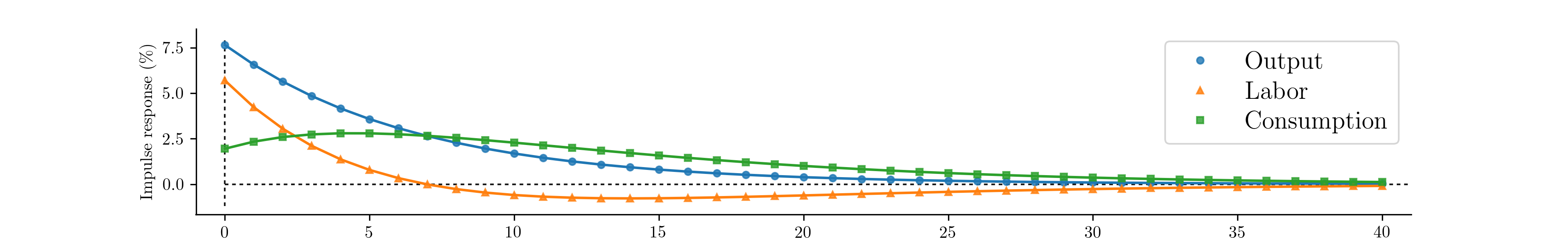
Fig. 8 Impulse response functions corresponding to a fully calibrated RBC model.
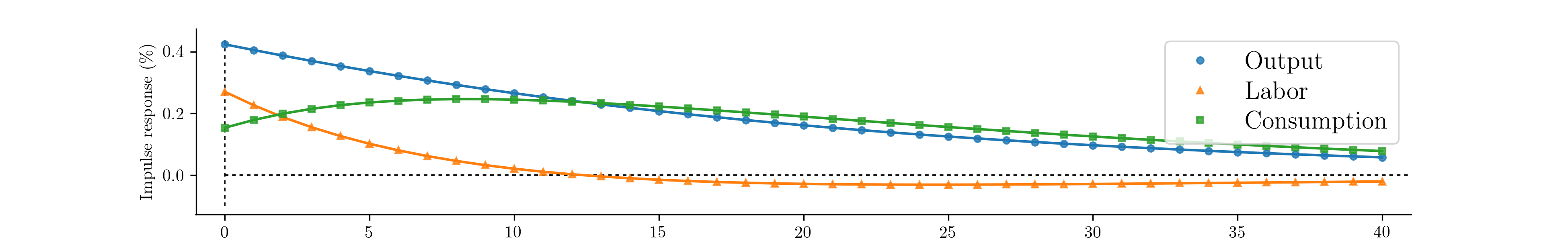
Fig. 9 Impulse response functions corresponding to a partially estimated RBC model.
Recall that the RBC model has three observables, output, labor, and consumption, and two unobserved states, capital and the technology process. The Kalman filter provides optimal estimates of these unobserved series at time \(t\) based on on all data up to time \(t\), and the state smoother provides optimal estimates based on the full dataset. These can be retrieved from the results object. Fig. 10 displays the smoothed state values and confidence intervals for the partially estimated case.
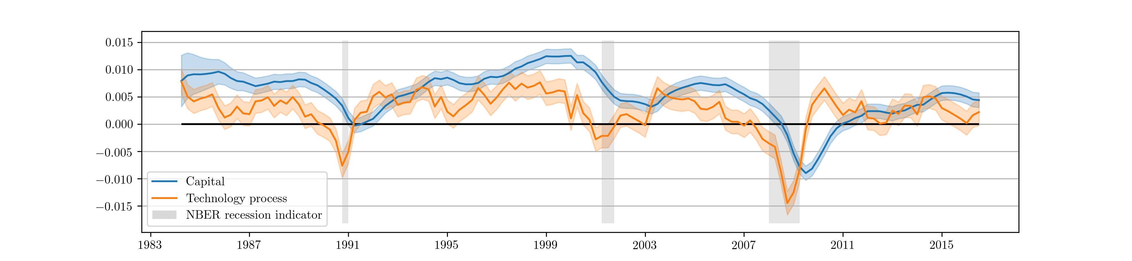
Fig. 10 Smoothed estimates of capital and the technology process from the partially estimated RBC model.
| [4] | We note again that this example is merely by way of illustration; it does not represent best-practices for careful RBC estimation. |