Implementing and estimating a simple Real Business Cycle (RBC) model(Open on Google Colab | View / download notebook | Report a problem)
This notebook collects the full example implementing and estimating (via maximum likelihood, Metropolis-Hastings, and Gibbs Sampling) a simple real business cycle model, from my working paper Estimating time series models by state space methods in Python: Statsmodels.
Table of Contents
Simple Real Business Cycle Model
This notebook contains the example code from “State Space Estimation of Time Series Models in Python: Statsmodels” for the simple RBC model.
# These are the basic import statements to get the required Python functionality
%matplotlib inline

import numpy as np
import pandas as pd
import statsmodels.api as sm
import matplotlib.pyplot as plt
Data
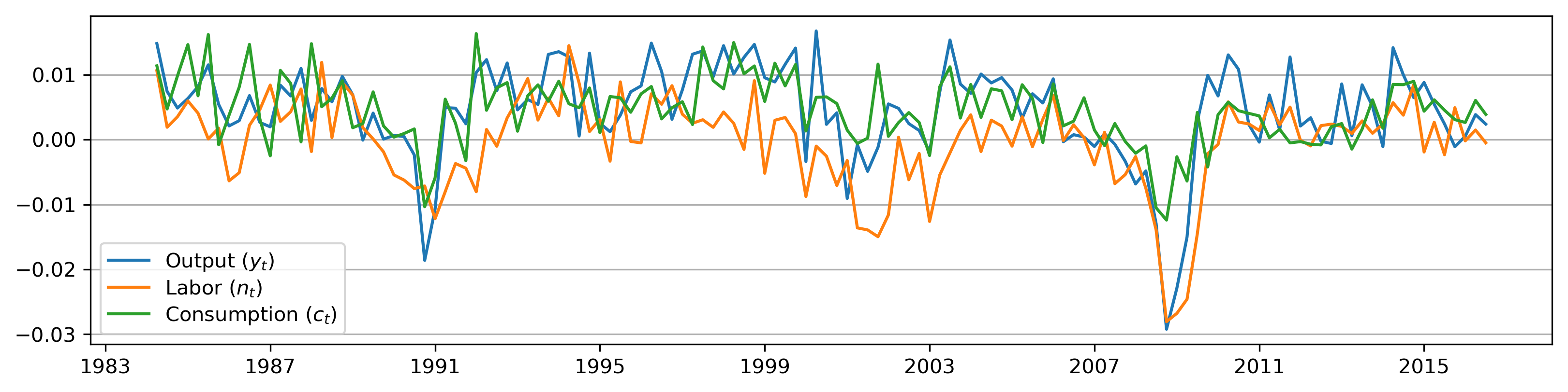
For this example, we consider an RBC model in which output, labor, and consumption are the observable series.
# RBC model
from pandas_datareader.data import DataReader
start = '1984-01'
end = '2016-09'
labor = DataReader('HOANBS', 'fred',start=start, end=end).resample('QS').first()
cons = DataReader('PCECC96', 'fred', start=start, end=end).resample('QS').first()
inv = DataReader('GPDIC1', 'fred', start=start, end=end).resample('QS').first()
pop = DataReader('CNP16OV', 'fred', start=start, end=end)
pop = pop.resample('QS').mean()  # Convert pop from monthly to quarterly observations
recessions = DataReader('USRECQ', 'fred', start=start, end=end)
recessions = recessions.resample('QS').last()['USRECQ'].iloc[1:]

# Get in per-capita terms
N = labor['HOANBS'] * 6e4 / pop['CNP16OV']
C = (cons['PCECC96'] * 1e6 / pop['CNP16OV']) / 4
I = (inv['GPDIC1'] * 1e6 / pop['CNP16OV']) / 4
Y = C + I

# Log, detrend
y = np.log(Y).diff()[1:]
c = np.log(C).diff()[1:]
n = np.log(N).diff()[1:]
i = np.log(I).diff()[1:]
rbc_data = pd.concat((y, n, c), axis=1)
rbc_data.columns = ['output', 'labor', 'consumption']
# Plot the series
fig, ax = plt.subplots(figsize=(13, 3), dpi=300)

ax.plot(y.index, y, label=r'Output $(y_t)$')
ax.plot(n.index, n, label=r'Labor $(n_t)$')
ax.plot(c.index, c, label=r'Consumption $(c_t)$')

ax.yaxis.grid()
ax.legend(loc='lower left', labelspacing=0.3);
RBC Model
The simple RBC model considered here can be found in Ruge-Murcia (2007) or Dejong and Dave (2011). The non-linear system of equilibrium conditions is as follows:
\[\begin{align} \psi c_t & = (1 - \alpha) z_t \left ( \frac{k_t}{n_t} \right )^{\alpha} & \text{Static FOC} \\ \frac{1}{c_t} & = \beta E_t \left \{ \frac{1}{c_{t+1}} \left [ \alpha z_{t+1} \left ( \frac{k_{t+1}}{n_{t+1}} \right )^{\alpha - 1} + (1 - \delta) \right ] \right \} & \text{Euler equation} \\ y_t & = z_t k_t^\alpha n_t^{1 - \alpha} & \text{Production function} \\ y_t & = c_t + i_t & \text{Aggregate resource constraint} \\ k_{t+1} & = (1 - \delta) k_t + i_t & \text{Captial accumulation} \\ 1 & = l_t + n_t & \text{Labor-leisure tradeoff} \\ \log z_t & = \rho \log z_{t-1} + \varepsilon_t & \text{Technology shock transition} \end{align}\]by linearizing the model around the non-stochastic steady state, reducing the system to the three variables above, and solving with the method of Blanchard and Kahn (1980), we achieve a model in state space form.
The class SimpleRBC, below, implements the log-linearization step in the log_linearize method and the Blanchard-Kahn solution in the solve method. The params vector for that class is the vector of structural parameters:
Also, the class below has a number of parameter transformations to ensure valid parameters. For example, transform_discount_rate takes as its argument a parameter that can vary over the entire real line and transformed it to lie in the set $(0, 1)$. This can be convenient when performing maximum likelihood estimation with some numerical optimization routines.
State space form
After log-linearizing and solving the model, the resultant state space form is:
\[\begin{align} \begin{bmatrix} y_t \\ n_t \\ c_t \end{bmatrix} & = \underbrace{\begin{bmatrix} \phi_{yk} & \phi_{yz} \\ \phi_{nk} & \phi_{nz} \\ \phi_{ck} & \phi_{cz} \\ \end{bmatrix}}_{Z} \underbrace{\begin{bmatrix} k_t \\ z_t \end{bmatrix}}_{\alpha_t} + \underbrace{\begin{bmatrix} \varepsilon_{y,t} \\ \varepsilon_{n,t} \\ \varepsilon_{c,t} \end{bmatrix}}_{\varepsilon_t}, \qquad \varepsilon_t \sim N \left ( \begin{bmatrix} 0 \\ 0 \\ 0\end{bmatrix}, \begin{bmatrix} \sigma_{y}^2 & 0 & 0 \\ 0 & \sigma_{n}^2 & 0 \\ 0 & 0 & \sigma_{c}^2 \\ \end{bmatrix} \right ) \\ \begin{bmatrix} k_{t+1} \\ z_{t+1} \end{bmatrix} & = \underbrace{\begin{bmatrix} T_{kk} & T_{kz} \\ 0 & \rho \end{bmatrix}}_{T} \begin{bmatrix} k_t \\ z_t \end{bmatrix} + \underbrace{\begin{bmatrix} 0 \\ 1 \end{bmatrix}}_{R} \eta_t, \qquad \eta_t \sim N(0, \sigma_z^2) \end{align}\]where the reduced form parameters in the state space model are non-linear functions of the parameters in the RBC model, above.
The update method is called with a params vector holding the structural parameters. By log-linearizing and solving the model, those sturctural parameters are transformed into the reduced form parameters making up the state space form, and these are placed into the design, obs_cov, transition, and state_cov matrices. Then the Kalman filter and smoother can be applied to retrieve smoothed estimates of the unobserved states, compute the log-likelihood for maximum likelihood estimation, or as part of the simulation smoother for Bayesian estimation.
x = OrderedDict()
x['a'] = 1
list(x.keys()).index('a')
0
from collections import OrderedDict
class SimpleRBC(sm.tsa.statespace.MLEModel):

    parameters = OrderedDict([
        ('discount_rate', 0.95),
        ('disutility_labor', 3.),
        ('depreciation_rate', 0.025),
        ('capital_share', 0.36),
        ('technology_shock_persistence', 0.85),
        ('technology_shock_var', 0.04**2)
    ])

    def __init__(self, endog, calibrated=None):
        super(SimpleRBC, self).__init__(
            endog, k_states=2, k_posdef=1, initialization='stationary')
        self.k_predetermined = 1

        # Save the calibrated vs. estimated parameters
        parameters = list(self.parameters.keys())
        calibrated = calibrated or {}
        self.calibrated = OrderedDict([
            (param, calibrated[param]) for param in parameters
            if param in calibrated
        ])
        self.idx_calibrated = np.array([
            param in self.calibrated for param in parameters])
        self.idx_estimated = ~self.idx_calibrated

        self.k_params = len(self.parameters)
        self.k_calibrated = len(self.calibrated)
        self.k_estimated = self.k_params - self.k_calibrated

        self.idx_cap_share = parameters.index('capital_share')
        self.idx_tech_pers = parameters.index('technology_shock_persistence')
        self.idx_tech_var = parameters.index('technology_shock_var')

        # Setup fixed elements of system matrices
        self['selection', 1, 0] = 1

    @property
    def start_params(self):
        structural_params = np.array(list(self.parameters.values()))[self.idx_estimated]
        measurement_variances = [0.1] * 3
        return np.r_[structural_params, measurement_variances]

    @property
    def param_names(self):
        structural_params = np.array(list(self.parameters.keys()))[self.idx_estimated]
        measurement_variances = ['%s.var' % name for name in self.endog_names]
        return structural_params.tolist() + measurement_variances

    def log_linearize(self, params):
        # Extract the parameters
        (discount_rate, disutility_labor, depreciation_rate, capital_share,
         technology_shock_persistence, technology_shock_var) = params

        # Temporary values
        tmp = (1. / discount_rate - (1. - depreciation_rate))
        theta = (capital_share / tmp)**(1. / (1. - capital_share))
        gamma = 1. - depreciation_rate * theta**(1. - capital_share)
        zeta = capital_share * discount_rate * theta**(capital_share - 1)

        # Coefficient matrices from linearization
        A = np.eye(2)

        B11 = 1 + depreciation_rate * (gamma / (1 - gamma))
        B12 = (-depreciation_rate *
               (1 - capital_share + gamma * capital_share) /
               (capital_share * (1 - gamma)))
        B21 = 0
        B22 = capital_share / (zeta + capital_share*(1 - zeta))
        B = np.array([[B11, B12], [B21, B22]])

        C1 = depreciation_rate / (capital_share * (1 - gamma))
        C2 = (zeta * technology_shock_persistence /
              (zeta + capital_share*(1 - zeta)))
        C = np.array([[C1], [C2]])

        return A, B, C

    def solve(self, params):
        capital_share = params[self.idx_cap_share]
        technology_shock_persistence = params[self.idx_tech_pers]

        # Get the coefficient matrices from linearization
        A, B, C = self.log_linearize(params)

        # Jordan decomposition of B
        eigvals, right_eigvecs = np.linalg.eig(np.transpose(B))
        left_eigvecs = np.transpose(right_eigvecs)

        # Re-order, ascending
        idx = np.argsort(eigvals)
        eigvals = np.diag(eigvals[idx])
        left_eigvecs = left_eigvecs[idx, :]

        # Blanchard-Kahn conditions
        k_nonpredetermined = self.k_states - self.k_predetermined
        k_stable = len(np.where(eigvals.diagonal() < 1)[0])
        k_unstable = self.k_states - k_stable
        if not k_stable == self.k_predetermined:
            raise RuntimeError('Blanchard-Kahn condition not met.'
                               ' Unique solution does not exist.')

        # Create partition indices
        k = self.k_predetermined
        p1 = np.s_[:k]
        p2 = np.s_[k:]

        p11 = np.s_[:k, :k]
        p12 = np.s_[:k, k:]
        p21 = np.s_[k:, :k]
        p22 = np.s_[k:, k:]

        # Decouple the system
        decoupled_C = np.dot(left_eigvecs, C)

        # Solve the explosive component (controls) in terms of the
        # non-explosive component (states) and shocks
        tmp = np.linalg.inv(left_eigvecs[p22])

        # This is \phi_{ck}, above
        policy_state = - np.dot(tmp, left_eigvecs[p21]).squeeze()
        # This is \phi_{cz}, above
        policy_shock = -(
            np.dot(tmp, 1. / eigvals[p22]).dot(
                np.linalg.inv(
                    np.eye(k_nonpredetermined) -
                    technology_shock_persistence / eigvals[p22]
                )
            ).dot(decoupled_C[p2])
        ).squeeze()

        # Solve for the non-explosive transition
        # This is T_{kk}, above
        transition_state = np.squeeze(B[p11] + np.dot(B[p12], policy_state))
        # This is T_{kz}, above
        transition_shock = np.squeeze(np.dot(B[p12], policy_shock) + C[p1])

        # Create the full design matrix
        tmp = (1 - capital_share) / capital_share
        tmp1 = 1. / capital_share
        design = np.array([[1 - tmp * policy_state, tmp1 - tmp * policy_shock],
                           [1 - tmp1 * policy_state, tmp1 * (1-policy_shock)],
                           [policy_state,            policy_shock]])

        # Create the transition matrix
        transition = (
            np.array([[transition_state, transition_shock],
                      [0,                technology_shock_persistence]]))

        return design, transition

    def transform_discount_rate(self, param, untransform=False):
        # Discount rate must be between 0 and 1
        epsilon = 1e-4  # bound it slightly away from exactly 0 or 1
        if not untransform:
            return np.abs(1 / (1 + np.exp(param)) - epsilon)
        else:
            return np.log((1 - param + epsilon) / (param + epsilon))

    def transform_disutility_labor(self, param, untransform=False):
        # Disutility of labor must be positive
        return param**2 if not untransform else param**0.5

    def transform_depreciation_rate(self, param, untransform=False):
        # Depreciation rate must be positive
        return param**2 if not untransform else param**0.5

    def transform_capital_share(self, param, untransform=False):
        # Capital share must be between 0 and 1
        epsilon = 1e-4  # bound it slightly away from exactly 0 or 1
        if not untransform:
            return np.abs(1 / (1 + np.exp(param)) - epsilon)
        else:
            return np.log((1 - param + epsilon) / (param + epsilon))

    def transform_technology_shock_persistence(self, param, untransform=False):
        # Persistence parameter must be between -1 and 1
        if not untransform:
            return param / (1 + np.abs(param))
        else:
            return param / (1 - param)

    def transform_technology_shock_var(self, unconstrained, untransform=False):
        # Variances must be positive
        return unconstrained**2 if not untransform else unconstrained**0.5

    def transform_params(self, unconstrained):
        constrained = np.zeros(unconstrained.shape, unconstrained.dtype)

        i = 0
        for param in self.parameters.keys():
            if param not in self.calibrated:
                method = getattr(self, 'transform_%s' % param)
                constrained[i] = method(unconstrained[i])
                i += 1

        # Measurement error variances must be positive
        constrained[self.k_estimated:] = unconstrained[self.k_estimated:]**2

        return constrained

    def untransform_params(self, constrained):
        unconstrained = np.zeros(constrained.shape, constrained.dtype)

        i = 0
        for param in self.parameters.keys():
            if param not in self.calibrated:
                method = getattr(self, 'transform_%s' % param)
                unconstrained[i] = method(constrained[i], untransform=True)
                i += 1

        # Measurement error variances must be positive
        unconstrained[self.k_estimated:] = constrained[self.k_estimated:]**0.5

        return unconstrained

    def update(self, params, **kwargs):
        params = super(SimpleRBC, self).update(params, **kwargs)

        # Reconstruct the full parameter vector from the
        # estimated and calibrated parameters
        structural_params = np.zeros(self.k_params, dtype=params.dtype)
        structural_params[self.idx_calibrated] = list(self.calibrated.values())
        structural_params[self.idx_estimated] = params[:self.k_estimated]
        measurement_variances = params[self.k_estimated:]

        # Solve the model
        design, transition = self.solve(structural_params)

        # Update the statespace representation
        self['design'] = design
        self['obs_cov', 0, 0] = measurement_variances[0]
        self['obs_cov', 1, 1] = measurement_variances[1]
        self['obs_cov', 2, 2] = measurement_variances[2]
        self['transition'] = transition
        self['state_cov', 0, 0] = structural_params[self.idx_tech_var]
Calibration / Maximum likelihood estimation
It is sometimes interesting to calibrate the structural parameters of the model, and estimate only the measurement error variables.
# Calibrate everything except measurement variances
calibrated = {
'discount_rate': 0.95,
'disutility_labor': 3.0,
'capital_share': 0.36,
'depreciation_rate': 0.025,
'technology_shock_persistence': 0.85,
'technology_shock_var': 0.04**2
}
calibrated_mod = SimpleRBC(rbc_data, calibrated=calibrated)
calibrated_res = calibrated_mod.fit(method='nm', maxiter=1000, disp=0)
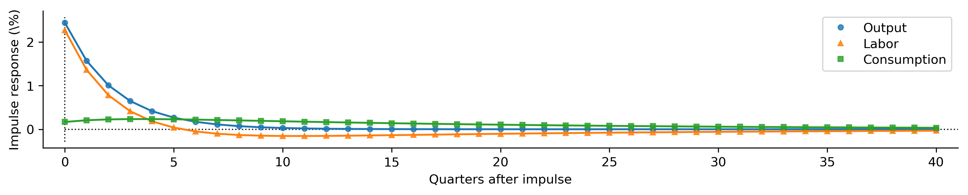
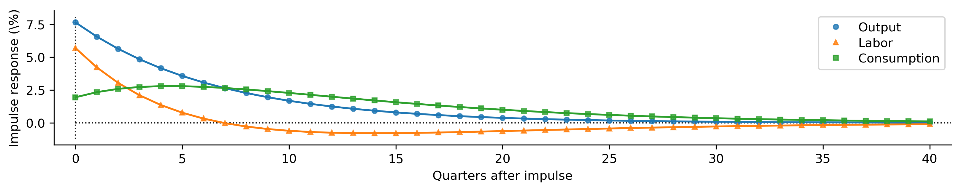
calibrated_irfs = calibrated_res.impulse_responses(40, orthogonalized=True) * 100
print(calibrated_res.summary())
                                   Statespace Model Results
==============================================================================================
Dep. Variable:     ['output', 'labor', 'consumption']   No. Observations:                  130
Model:                                      SimpleRBC   Log Likelihood                1226.745
Date:                                Thu, 01 Nov 2018   AIC                          -2447.489
Time:                                        20:35:50   BIC                          -2438.887
Sample:                                    04-01-1984   HQIC                         -2443.994
                                         - 07-01-2016
Covariance Type:                                  opg
===================================================================================
                      coef    std err          z      P>|z|      [0.025      0.975]
-----------------------------------------------------------------------------------
output.var       6.449e-10   6.12e-06      0.000      1.000    -1.2e-05     1.2e-05
labor.var        3.783e-05   4.18e-06      9.054      0.000    2.96e-05     4.6e-05
consumption.var  1.462e-05   1.79e-06      8.166      0.000    1.11e-05    1.81e-05
=====================================================================================
Ljung-Box (Q):          46.67, 140.06, 52.77   Jarque-Bera (JB):    6.89, 13.51, 7.85
Prob(Q):                    0.22, 0.00, 0.09   Prob(JB):             0.03, 0.00, 0.02
Heteroskedasticity (H):     1.24, 1.14, 0.47   Skew:               -0.08, -0.61, 0.53
Prob(H) (two-sided):        0.48, 0.66, 0.02   Kurtosis:             4.12, 3.99, 3.59
=====================================================================================

Warnings:
[1] Covariance matrix calculated using the outer product of gradients (complex-step).
Output plots
Because we’re going to be making the same plots for a couple of examples, we define a function here to do that for us.
from scipy.stats import norm
def plot_irfs(irfs):
fig, ax = plt.subplots(figsize=(13, 2), dpi=300)
lines, = ax.plot(irfs['output'], label='')
ax.plot(irfs['output'], 'o', label='Output', color=lines.get_color(),
markersize=4, alpha=0.8)
lines, = ax.plot(irfs['labor'], label='')
ax.plot(irfs['labor'], '^', label='Labor', color=lines.get_color(),
markersize=4, alpha=0.8)
lines, = ax.plot(irfs['consumption'], label='')
ax.plot(irfs['consumption'], 's', label='Consumption',
color=lines.get_color(), markersize=4, alpha=0.8)
ax.hlines(0, 0, irfs.shape[0], alpha=0.9, linestyle=':', linewidth=1)
ylim = ax.get_ylim()
ax.vlines(0, ylim[0]+1e-6, ylim[1]-1e-6, alpha=0.9, linestyle=':',
linewidth=1)
[ax.spines[spine].set(linewidth=0) for spine in ['top', 'right']]
ax.set(xlabel='Quarters after impulse', ylabel='Impulse response (\%)',
xlim=(-1, len(irfs)))
ax.legend(labelspacing=0.3)
return fig
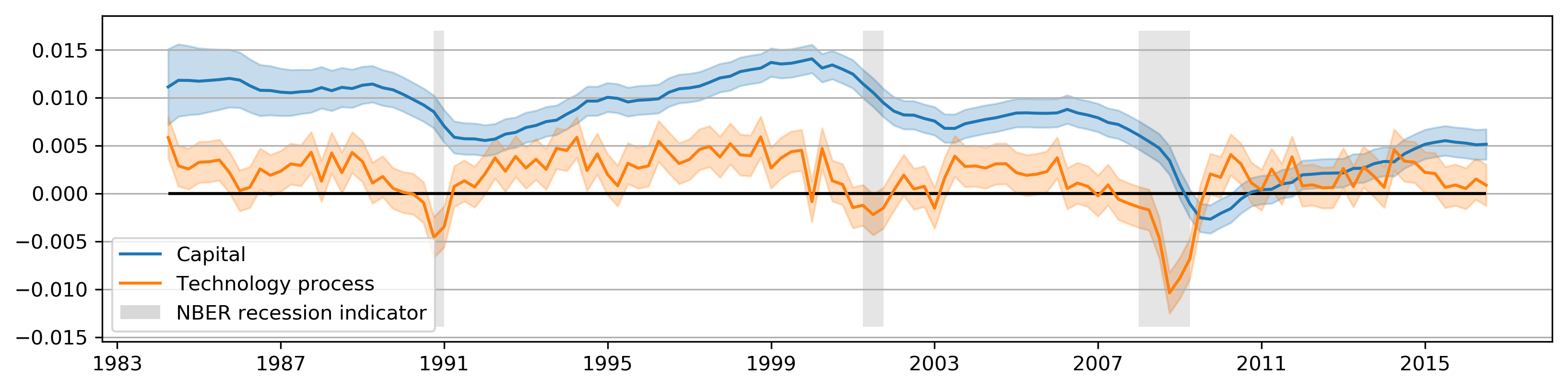
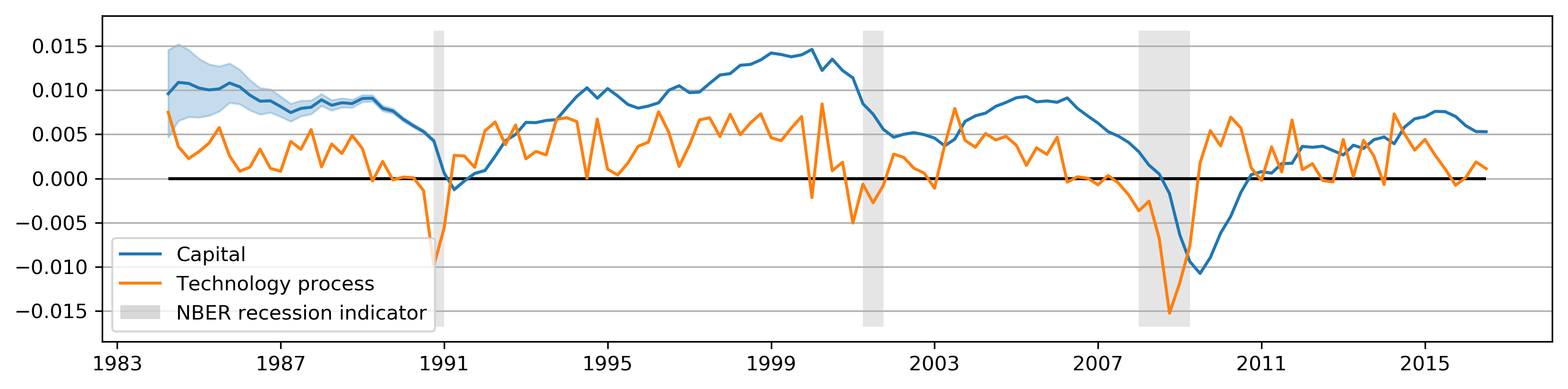
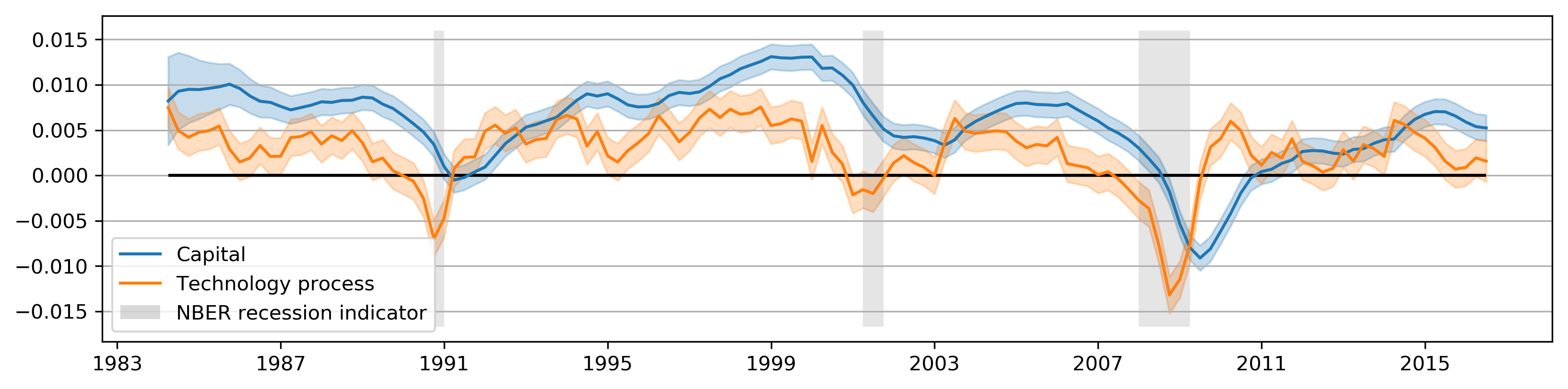
def plot_states(res):
fig, ax = plt.subplots(figsize=(13, 3), dpi=300)
alpha = 0.1
q = norm.ppf(1 - alpha / 2)
capital = res.smoothed_state[0, :]
capital_se = res.smoothed_state_cov[0, 0, :]**0.5
capital_lower = capital - capital_se * q
capital_upper = capital + capital_se * q
shock = res.smoothed_state[1, :]
shock_se = res.smoothed_state_cov[1, 1, :]**0.5
shock_lower = shock - shock_se * q
shock_upper = shock + shock_se * q
line_capital, = ax.plot(rbc_data.index, capital, label='Capital')
ax.fill_between(rbc_data.index, capital_lower, capital_upper, alpha=0.25,
color=line_capital.get_color())
line_shock, = ax.plot(rbc_data.index, shock, label='Technology process')
ax.fill_between(rbc_data.index, shock_lower, shock_upper, alpha=0.25,
color=line_shock.get_color())
ax.hlines(0, rbc_data.index[0], rbc_data.index[-1], 'k')
ax.yaxis.grid()
ylim = ax.get_ylim()
ax.fill_between(recessions.index, ylim[0]+1e-5, ylim[1]-1e-5, recessions,
facecolor='k', alpha=0.1)
p1 = plt.Rectangle((0, 0), 1, 1, fc="grey", alpha=0.3)
ax.legend([line_capital, line_shock, p1],
["Capital", "Technology process", "NBER recession indicator"],
loc='lower left');
return fig
plot_states(calibrated_res);
plot_irfs(calibrated_irfs);
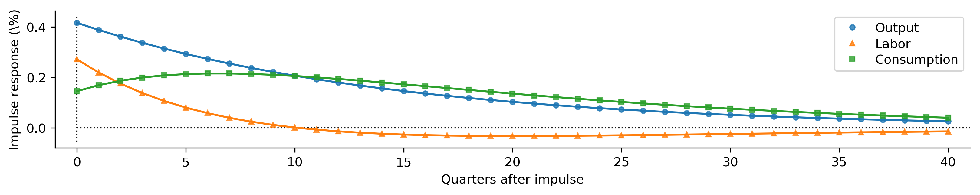
Maximum likelihood estimation
We can try to estimate more parameters.
# Now, don't calibrate the technology parameters
partially_calibrated = {
    'discount_rate': 0.95,
    'disutility_labor': 3.0,
    'capital_share': 0.33,
    'depreciation_rate': 0.025,
}
partial_mod = SimpleRBC(rbc_data, calibrated=partially_calibrated)
partial_res = partial_mod.fit(method='nm', maxiter=1000, disp=0)

partial_irfs = partial_res.impulse_responses(40, orthogonalized=True) * 100
print(partial_res.summary())
                                   Statespace Model Results
==============================================================================================
Dep. Variable:     ['output', 'labor', 'consumption']   No. Observations:                  130
Model:                                      SimpleRBC   Log Likelihood                1501.123
Date:                                Thu, 01 Nov 2018   AIC                          -2992.246
Time:                                        20:35:53   BIC                          -2977.908
Sample:                                    04-01-1984   HQIC                         -2986.420
                                         - 07-01-2016
Covariance Type:                                  opg
================================================================================================
                                   coef    std err          z      P>|z|      [0.025      0.975]
------------------------------------------------------------------------------------------------
technology_shock_persistence     0.9329      0.023     40.397      0.000       0.888       0.978
technology_shock_var          5.491e-06   1.04e-06      5.277      0.000    3.45e-06    7.53e-06
output.var                    9.967e-06   2.67e-06      3.731      0.000    4.73e-06    1.52e-05
labor.var                      3.33e-05   4.31e-06      7.730      0.000    2.49e-05    4.17e-05
consumption.var               1.444e-05   1.64e-06      8.817      0.000    1.12e-05    1.77e-05
======================================================================================
Ljung-Box (Q):          35.57, 193.85, 53.19   Jarque-Bera (JB):   12.25, 11.14, 16.40
Prob(Q):                    0.67, 0.00, 0.08   Prob(JB):              0.00, 0.00, 0.00
Heteroskedasticity (H):     1.36, 1.19, 0.50   Skew:                 0.14, -0.61, 0.69
Prob(H) (two-sided):        0.31, 0.58, 0.03   Kurtosis:              4.48, 3.75, 4.07
======================================================================================

Warnings:
[1] Covariance matrix calculated using the outer product of gradients (complex-step).
plot_states(partial_res);
plot_irfs(partial_irfs);
Metropolis-within-Gibbs Sampling
def draw_posterior_rho(model, states, sigma2, truncate=False):
    Z = states[1:2, 1:]
    X = states[1:2, :-1]

    tmp = 1 / (sigma2 + np.sum(X**2))
    post_mean = tmp * np.squeeze(np.dot(X, Z.T))
    post_var = tmp * sigma2

    if truncate:
        lower = (-1 - post_mean) / post_var**0.5
        upper = (1 - post_mean) / post_var**0.5
        rvs = truncnorm.rvs(lower, upper, loc=post_mean, scale=post_var**0.5)
    else:
        rvs = norm.rvs(post_mean, post_var**0.5)
    return rvs

def draw_posterior_sigma2(model, states, rho):
    resid = states[1, 1:] - rho * states[1, :-1]
    post_shape = 2.00005 + model.nobs
    post_scale = 0.0100005 + np.sum(resid**2)

    return invgamma.rvs(post_shape, scale=post_scale)

np.set_printoptions(suppress=True)
np.random.seed(17429)

from statsmodels.tsa.statespace.tools import is_invertible
from scipy.stats import multivariate_normal, gamma, invgamma, beta, uniform

# Create the model for likelihood evaluation
calibrated = {
    'disutility_labor': 3.0,
    'depreciation_rate': 0.025,
}
model = SimpleRBC(rbc_data, calibrated=calibrated)
sim_smoother = model.simulation_smoother()

# Specify priors
prior_discount = gamma(6.25, scale=0.04)
prior_cap_share = norm(0.3, scale=0.01)
prior_meas_err = invgamma(2.0025, scale=0.10025)

# Proposals
rw_discount = norm(scale=0.3)
rw_cap_share = norm(scale=0.01)
rw_meas_err = norm(scale=0.003)

# Create storage arrays for the traces
n_iterations = 10000
trace = np.zeros((n_iterations + 1, 7))
trace_accepts = np.zeros((n_iterations, 5))
trace[0] = model.start_params
trace[0, 0] = 100 * ((1 / trace[0, 0]) - 1)

loglike = None

# Iterations
for s in range(1, n_iterations + 1):
    if s % 1000 == 0:
        print(s)
    # Get the parameters from the trace
    discount_rate = 1 / (1 + (trace[s-1, 0] / 100))
    capital_share = trace[s-1, 1]
    rho = trace[s-1, 2]
    sigma2 = trace[s-1, 3]
    meas_vars = trace[s-1, 4:]**2

    # 1. Gibbs step: draw the states using the simulation smoother
    model.update(np.r_[discount_rate, capital_share, rho, sigma2, meas_vars])
    sim_smoother.simulate()
    states = sim_smoother.simulated_state[:, :-1]

    # 2. Gibbs step: draw the autoregressive parameter, and apply
    # rejection sampling to ensure an invertible lag polynomial
    # In rare cases due to the combinations of other parameters,
    # the mean of the normal posterior will be greater than one
    # and it becomes difficult to draw from a normal distribution
    # even with rejection sampling. In those cases we draw from a
    # truncated normal.
    rho = draw_posterior_rho(model, states, sigma2)
    i = 0
    while rho < -1 or rho > 1:
        if i < 1e2:
            rho = draw_posterior_rho(model, states, sigma2)
        else:
            rho = draw_posterior_rho(model, states, sigma2, truncate=True)
        i += 1
    trace[s, 2] = rho

    # 3. Gibbs step: draw the variance parameter
    sigma2 = draw_posterior_sigma2(model, states, rho)
    trace[s, 3] = sigma2

    # Calculate the loglikelihood
    loglike = model.loglike(np.r_[discount_rate, capital_share, rho, sigma2, meas_vars])

    # 4. Metropolis-step for the discount rate
    discount_param = trace[s-1, 0]
    proposal_param = discount_param + rw_discount.rvs()
    proposal_rate = 1 / (1 + (proposal_param / 100))
    if proposal_rate < 1:
        proposal_loglike = model.loglike(np.r_[proposal_rate, capital_share, rho, sigma2, meas_vars])
        acceptance_probability = np.exp(
            proposal_loglike - loglike +
            prior_discount.logpdf(proposal_param) -
            prior_discount.logpdf(discount_param))

        if acceptance_probability > uniform.rvs():
            discount_param = proposal_param
            discount_rate = proposal_rate
            loglike = proposal_loglike
            trace_accepts[s-1, 0] = 1

    trace[s, 0] = discount_param

    # 5. Metropolis-step for the capital-share
    proposal = capital_share + rw_cap_share.rvs()
    if proposal > 0 and proposal < 1:
        proposal_loglike = model.loglike(np.r_[discount_rate, proposal, rho, sigma2, meas_vars])
        acceptance_probability = np.exp(
            proposal_loglike - loglike +
            prior_cap_share.logpdf(proposal) -
            prior_cap_share.logpdf(capital_share))

        if acceptance_probability > uniform.rvs():
            capital_share = proposal
            trace_accepts[s-1, 1] = 1
            loglike = proposal_loglike
    trace[s, 1] = capital_share

    # 6. Metropolis-step for the measurement errors
    for i in range(3):
        meas_std = meas_vars[i]**0.5
        proposal = meas_std + rw_meas_err.rvs()
        proposal_vars = meas_vars.copy()
        proposal_vars[i] = proposal**2
        if proposal > 0:
            proposal_loglike = model.loglike(np.r_[discount_rate, capital_share, rho, sigma2, proposal_vars])
            acceptance_probability = np.exp(
                proposal_loglike - loglike +
                prior_meas_err.logpdf(proposal) -
                prior_meas_err.logpdf(meas_std))

            if acceptance_probability > uniform.rvs():
                meas_std = proposal
                trace_accepts[s-1, 2+i] = 1
                loglike = proposal_loglike
                meas_vars[i] = proposal_vars[i]
        trace[s, 4+i] = meas_std
1000
2000
3000
4000
5000
6000
7000
8000
9000
10000
from scipy.stats import gaussian_kde

burn = 1000
thin = 10

final_trace = trace.copy()
final_trace = final_trace[burn:][::thin]
final_trace[:, 0] = 1 / (1 + (final_trace[:, 0] / 100))
final_trace[:, 4:] = final_trace[:, 4:]**2

modes = np.zeros(7)
means = np.mean(final_trace, axis=0)
discount_kde = gaussian_kde(final_trace[:, 0])
cap_share_kde = gaussian_kde(final_trace[:, 1])
rho_kde = gaussian_kde(final_trace[:, 2])
sigma2_kde = gaussian_kde(final_trace[:, 3])

# Finish calculating modes
for i in range(7):
    kde = gaussian_kde(final_trace[:, i])
    X = np.linspace(np.min(final_trace[:, i]),
                    np.max(final_trace[:, i]), 1000)
    Y = kde(X)
    modes[i] = X[np.argmax(Y)]

test = pd.DataFrame(final_trace)

print(pd.DataFrame(
    np.c_[modes, means, test.quantile(q=0.05), test.quantile(q=0.95)],
    columns=['Mode', 'Mean', '5 percent', '95 percent']
).to_string(float_format=lambda x: '%.3g' % x))
      Mode     Mean  5 percent  95 percent
0    0.997    0.996      0.994       0.998
1     0.33    0.327      0.311       0.344
2    0.674    0.625      0.263       0.927
3 8.21e-05 8.34e-05   7.12e-05    9.75e-05
4    2e-05 2.07e-05   1.37e-05    2.97e-05
5 2.83e-05 2.95e-05   2.05e-05       4e-05
6 2.27e-05 2.38e-05   1.81e-05    3.01e-05
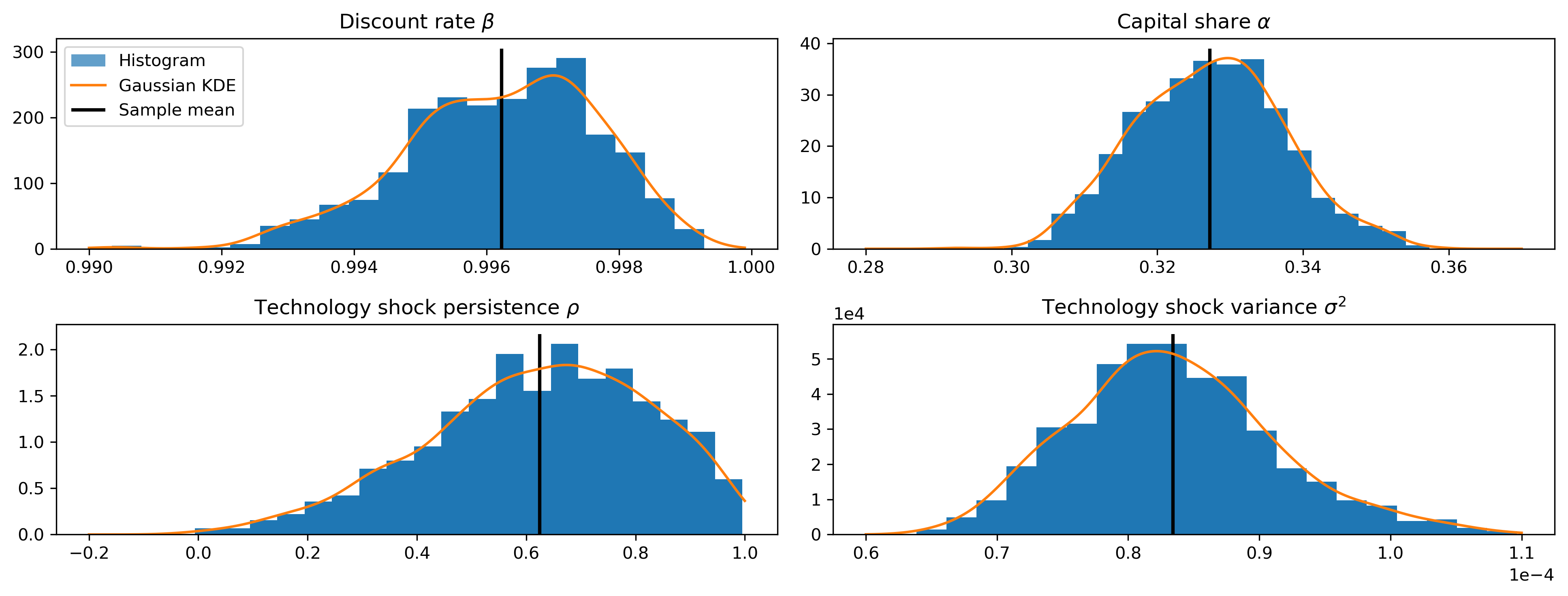
Sampler output
# Trace plots
fig, axes = plt.subplots(2, 2, figsize=(13, 5), dpi=300)

axes[0, 0].hist(final_trace[:, 0], bins=20, density=True, alpha=1)
X = np.linspace(0.990, 1.0-1e-4, 1000)
Y = discount_kde(X)
modes[0] = X[np.argmax(Y)]
line, = axes[0, 0].plot(X, Y)
ylim = axes[0, 0].get_ylim()
vline = axes[0, 0].vlines(means[0], ylim[0], ylim[1], linewidth=2)
axes[0, 0].set(title=r'Discount rate $\beta$')

axes[0, 1].hist(final_trace[:, 1], bins=20, density=True, alpha=1)
X = np.linspace(0.280, 0.370, 1000)
Y = cap_share_kde(X)
modes[1] = X[np.argmax(Y)]
axes[0, 1].plot(X, Y)
ylim = axes[0, 1].get_ylim()
vline = axes[0, 1].vlines(means[1], ylim[0], ylim[1], linewidth=2)
axes[0, 1].set(title=r'Capital share $\alpha$')

axes[1, 0].hist(final_trace[:, 2], bins=20, density=True, alpha=1)
X = np.linspace(-0.2, 1-1e-4, 1000)
Y = rho_kde(X)
modes[2] = X[np.argmax(Y)]
axes[1, 0].plot(X, Y)
ylim = axes[1, 0].get_ylim()
vline = axes[1, 0].vlines(means[2], ylim[0], ylim[1], linewidth=2)
axes[1, 0].set(title=r'Technology shock persistence $\rho$')

axes[1, 1].hist(final_trace[:, 3], bins=20, density=True, alpha=1)
X = np.linspace(0.6e-4, 1.1e-4, 1000)
Y = sigma2_kde(X)
modes[3] = X[np.argmax(Y)]
axes[1, 1].plot(X, Y)
ylim = axes[1, 1].get_ylim()
vline = axes[1, 1].vlines(means[3], ylim[0], ylim[1], linewidth=2)
axes[1, 1].ticklabel_format(style='sci', scilimits=(-2, 2))
axes[1, 1].set(title=r'Technology shock variance $\sigma^2$')

p1 = plt.Rectangle((0, 0), 1, 1, alpha=0.7)
axes[0, 0].legend([p1, line, vline],
                  ["Histogram", "Gaussian KDE", "Sample mean"],
                  loc='upper left')
fig.tight_layout()
Model of the posterior median
One way to explore the implications of the posterior is to example the model at the posterior mean or median.
gibbs_res = model.smooth(np.median(final_trace, axis=0))
print(gibbs_res.summary())

gibbs_irfs = gibbs_res.impulse_responses(40, orthogonalized=True)*100
                                   Statespace Model Results
==============================================================================================
Dep. Variable:     ['output', 'labor', 'consumption']   No. Observations:                  130
Model:                                      SimpleRBC   Log Likelihood                1353.026
Date:                                Thu, 01 Nov 2018   AIC                          -2692.052
Time:                                        20:38:30   BIC                          -2671.979
Sample:                                    04-01-1984   HQIC                         -2683.895
                                         - 07-01-2016
Covariance Type:                                  opg
================================================================================================
                                   coef    std err          z      P>|z|      [0.025      0.975]
------------------------------------------------------------------------------------------------
discount_rate                    0.9963      0.008    118.930      0.000       0.980       1.013
capital_share                    0.3274      0.179      1.833      0.067      -0.023       0.677
technology_shock_persistence     0.6423      0.390      1.648      0.099      -0.122       1.406
technology_shock_var          8.303e-05   7.43e-05      1.117      0.264   -6.27e-05       0.000
output.var                    2.017e-05   2.09e-05      0.964      0.335   -2.08e-05    6.12e-05
labor.var                     2.909e-05   1.85e-05      1.570      0.116   -7.22e-06    6.54e-05
consumption.var               2.363e-05   4.14e-06      5.704      0.000    1.55e-05    3.18e-05
=====================================================================================
Ljung-Box (Q):          35.26, 72.73, 58.06   Jarque-Bera (JB):     16.34, 0.66, 2.89
Prob(Q):                   0.68, 0.00, 0.03   Prob(JB):              0.00, 0.72, 0.24
Heteroskedasticity (H):    1.25, 0.83, 0.58   Skew:               -0.32, -0.11, -0.24
Prob(H) (two-sided):       0.47, 0.54, 0.08   Kurtosis:              4.62, 3.28, 3.55
=====================================================================================

Warnings:
[1] Covariance matrix calculated using the outer product of gradients (complex-step).
plot_states(gibbs_res);
plot_irfs(gibbs_irfs);