Estimating a Real Business Cycle DSGE Model by Maximum Likelihood in Python(Open on Google Colab | View / download notebook | Report a problem)
Note: this page was updated on October 26, 2016.
Table of Contents
Estimating a Real Business Cycle DSGE Model by Maximum Likelihood in Python
This notebook demonstrates how to setup, solve, and estimate a simple real business cycle model in Python. The model is very standard; the setup and notation here is a hybrid of Ruge-Murcia (2007) and DeJong and Dave (2011).
Since we will be proceeding step-by-step, the code will match that progression by generating a series of child classes, so that we can add the functionality step-by-step. Of course, in practice a single class incorporating all the functionality would be all you would need.
%matplotlib inline
from __future__ import division

import numpy as np
from scipy import optimize, signal
import pandas as pd
from pandas_datareader.data import DataReader
import statsmodels.api as sm
from statsmodels.tools.numdiff import approx_fprime, approx_fprime_cs
from IPython.display import display
import matplotlib.pyplot as plt
# import seaborn as sn

from numpy.testing import assert_allclose

# Set some pretty-printing options
np.set_printoptions(precision=3, suppress=True, linewidth=120)
pd.set_option('float_format', lambda x: '%.3g' % x, )
Household problem
\[\max E_0 \sum_{t=0}^\infty \beta^t u(c_t, l_t)\]subject to:
- the budget constraint: $y_t = c_t + i_t$
- the capital accumulation equation: $k_{t+1} = (1 - \delta) k_t + i_t$
- $1 = l_t + n_t$
where households have the following production technology:
\[y_t = z_t f(k_t, n_t)\]and where the (log of the) technology process follows an AR(1) process:
\[\log z_t = \rho \log z_{t-1} + \varepsilon_t, \qquad \varepsilon_t \sim N(0, \sigma^2)\]Functional forms
We will assume additively separable utility in consumption and leisure, with:
\[u(c_t, n_t) = \log(c_t) + \psi l_t\]where $\psi$ is a scalar weight.
The production function will be Cobb-Douglas:
\[f(k_t, n_t) = k_t^\alpha n_t^{1 - \alpha}\]Optimal behavior
Optimal household behavior is standard:
\[\begin{align} \psi & = \frac{1}{c_t} (1 - \alpha) z_t \left ( \frac{k_t}{n_t} \right )^{\alpha} \\ \frac{1}{c_t} & = \beta E_t \left \{ \frac{1}{c_{t+1}} \left [ \alpha z_{t+1} \left ( \frac{k_{t+1}}{n_{t+1}} \right )^{\alpha - 1} + (1 - \delta) \right ] \right \} \\ \end{align}\]Nonlinear system
Collecting all of the model equations, we have:
\[\begin{align} \psi c_t & = (1 - \alpha) z_t \left ( \frac{k_t}{n_t} \right )^{\alpha} & \text{Static FOC} \\ \frac{1}{c_t} & = \beta E_t \left \{ \frac{1}{c_{t+1}} \left [ \alpha z_{t+1} \left ( \frac{k_{t+1}}{n_{t+1}} \right )^{\alpha - 1} + (1 - \delta) \right ] \right \} & \text{Euler equation} \\ y_t & = z_t k_t^\alpha n_t^{1 - \alpha} & \text{Production function} \\ y_t & = c_t + i_t & \text{Aggregate resource constraint} \\ k_{t+1} & = (1 - \delta) k_t + i_t & \text{Captial accumulation} \\ 1 & = l_t + n_t & \text{Labor-leisure tradeoff} \\ \log z_t & = \rho \log z_{t-1} + \varepsilon_t & \text{Technology shock transition} \end{align}\]Variables / Parameters
This system is in the following variables:
\[\begin{align} x_t = \{ \quad & &\\ & y_t, & \text{Output}\\ & c_t, & \text{Consumption}\\ & i_t, & \text{Investment}\\ & n_t, & \text{Labor}\\ & l_t, & \text{Leisure}\\ & k_t, & \text{Capital}\\ & z_t & \text{Technology} \\ \} \quad & & \end{align}\]and depends on the following parameters:
\[\begin{align} \{ \quad & &\\ & \beta, & \text{Discount rate}\\ & \psi, & \text{Marginal disutility of labor}\\ & \delta, & \text{Depreciation rate}\\ & \alpha, & \text{Capital-share of output}\\ & \rho, & \text{Technology shock persistence}\\ & \sigma^2 & \text{Technology shock variance}\\ \} \quad & & \end{align}\]# Save the names of the equations, variables, and parameters
equation_names = [
'static FOC', 'euler equation', 'production',
'aggregate resource constraint', 'capital accumulation',
'labor-leisure', 'technology shock transition'
]
variable_names = [
'output', 'consumption', 'investment',
'labor', 'leisure', 'capital', 'technology'
]
parameter_names = [
'discount rate', 'marginal disutility of labor',
'depreciation rate', 'capital share',
'technology shock persistence',
'technology shock standard deviation',
]
# Save some symbolic forms for pretty-printing
variable_symbols = [
r"y", r"c", r"i", r"n", r"l", r"k", r"z",
]
contemporaneous_variable_symbols = [
r"$%s_t$" % symbol for symbol in variable_symbols
]
lead_variable_symbols = [
r"$%s_{t+1}$" % symbol for symbol in variable_symbols
]
parameter_symbols = [
r"$\beta$", r"$\psi$", r"$\delta$", r"$\alpha$", r"$\rho$", r"$\sigma^2$"
]
Numerical method
Using these equations, we can numerically find the steady-state using a root-finding algorithm and can then log-linearize around the steady-state using a numerical gradient procedure. In particular, here we follow DeJong and Dave (2011) chapter 2 and 3.1.
Write the generic non-linear system as:
\[\Gamma(E_t x_{t+1}, x_t, z_t) = 0\]in the absense of shocks, this can be rewritten as:
\[\Psi(x_{t+1}, x_t) = 0\]or as:
\[\Psi_1(x_{t+1}, x_t) = \Psi_2(x_{t+1}, x_t)\]and finally in logs as
\[\log \Psi_1(e^{\log x_{t+1}}, e^{\log x_t}) - \log \Psi_2(e^{\log x_{t+1}}, e^{\log x_t}) = 0\]First, we define a new class (RBC1) which holds the state of the RBC model (its dimensions, parameters, etc) and has methods for evaluating the log system. The eval_logged method evaluates the last equation, above.
Notice that the order of variables and order of equations is as described above.
class RBC1(object):
    def __init__(self, params=None):
        # Model dimensions
        self.k_params = 6
        self.k_variables = 7

        # Initialize parameters
        if params is not None:
            self.update(params)

    def update(self, params):
        # Save deep parameters
        self.discount_rate = params[0]
        self.disutility_labor = params[1]
        self.depreciation_rate = params[2]
        self.capital_share = params[3]
        self.technology_shock_persistence = params[4]
        self.technology_shock_std = params[5]

    def eval_logged(self, log_lead, log_contemporaneous):
        (log_lead_output, log_lead_consumption, log_lead_investment,
         log_lead_labor, log_lead_leisure, log_lead_capital,
         log_lead_technology_shock) = log_lead

        (log_output, log_consumption, log_investment, log_labor,
         log_leisure, log_capital, log_technology_shock) = log_contemporaneous

        return np.r_[
            self.log_static_foc(
                log_lead_consumption, log_lead_labor,
                log_lead_capital, log_lead_technology_shock
            ),
            self.log_euler_equation(
                log_lead_consumption, log_lead_labor,
                log_lead_capital, log_lead_technology_shock,
                log_consumption
            ),
            self.log_production(
                log_lead_output, log_lead_labor, log_lead_capital,
                log_lead_technology_shock
            ),
            self.log_aggregate_resource_constraint(
                log_lead_output, log_lead_consumption,
                log_lead_investment
            ),
            self.log_capital_accumulation(
                log_lead_capital, log_investment, log_capital
            ),
            self.log_labor_leisure_constraint(
                log_lead_labor, log_lead_leisure
            ),
            self.log_technology_shock_transition(
                log_lead_technology_shock, log_technology_shock
            )
        ]

    def log_static_foc(self, log_lead_consumption, log_lead_labor,
                       log_lead_capital, log_lead_technology_shock):
        return (
            np.log(self.disutility_labor) +
            log_lead_consumption -
            np.log(1 - self.capital_share) -
            log_lead_technology_shock -
            self.capital_share * (log_lead_capital - log_lead_labor)
        )

    def log_euler_equation(self, log_lead_consumption, log_lead_labor,
                           log_lead_capital, log_lead_technology_shock,
                           log_consumption):
        return (
            -log_consumption -
            np.log(self.discount_rate) +
            log_lead_consumption -
            np.log(
                (self.capital_share *
                 np.exp(log_lead_technology_shock) *
                 np.exp((1 - self.capital_share) * log_lead_labor) /
                 np.exp((1 - self.capital_share) * log_lead_capital)) +
                (1 - self.depreciation_rate)
            )
        )

    def log_production(self, log_lead_output, log_lead_labor, log_lead_capital,
                       log_lead_technology_shock):
        return (
            log_lead_output -
            log_lead_technology_shock -
            self.capital_share * log_lead_capital -
            (1 - self.capital_share) * log_lead_labor
        )

    def log_aggregate_resource_constraint(self, log_lead_output, log_lead_consumption,
                                          log_lead_investment):
        return (
            log_lead_output -
            np.log(np.exp(log_lead_consumption) + np.exp(log_lead_investment))
        )

    def log_capital_accumulation(self, log_lead_capital, log_investment, log_capital):
        return (
            log_lead_capital -
            np.log(np.exp(log_investment) + (1 - self.depreciation_rate) * np.exp(log_capital))
        )

    def log_labor_leisure_constraint(self, log_lead_labor, log_lead_leisure):
        return (
            -np.log(np.exp(log_lead_labor) + np.exp(log_lead_leisure))
        )

    def log_technology_shock_transition(self, log_lead_technology_shock, log_technology_shock):
        return (
            log_lead_technology_shock -
            self.technology_shock_persistence * log_technology_shock
        )
Later we will estimate (some of) the parameters; in the meantime we fix them at the values used to generate the datasets in Ruge-Murcia (2007).
# Setup fixed parameters
parameters = pd.DataFrame({
    'name': parameter_names,
    'value': [0.95, 3, 0.025, 0.36, 0.85, 0.04]
})
parameters.T
| 0 | 1 | 2 | 3 | 4 | 5 | |
|---|---|---|---|---|---|---|
| name | discount rate | marginal disutility of labor | depreciation rate | capital share | technology shock persistence | technology shock standard deviation |
| value | 0.95 | 3 | 0.025 | 0.36 | 0.85 | 0.04 |
Steady state
Numeric calculation
To numerically calculate steady-state, we apply a root-finding algorithm to the eval_logged method. In particular, we are finding values $\bar x$ such that
These will be confirmed analytically, below.
Here we create a derived class, RBC2 which extends all of the functionality from above, but now includes methods for numerical calcualtion of the steady-state.
class RBC2(RBC1):
    def steady_state_numeric(self):
        # Setup starting parameters
        log_start_vars = [0.5] * self.k_variables  # very arbitrary

        # Setup the function the evaluate
        eval_logged = lambda log_vars: self.eval_logged(log_vars, log_vars)

        # Apply the root-finding algorithm
        result = optimize.root(eval_logged, log_start_vars)

        return np.exp(result.x)

mod2 = RBC2(parameters['value'])

steady_state = pd.DataFrame({
    'value': mod2.steady_state_numeric()
}, index=variable_names)

steady_state.T
| output | consumption | investment | labor | leisure | capital | technology | |
|---|---|---|---|---|---|---|---|
| value | 0.572 | 0.506 | 0.0663 | 0.241 | 0.759 | 2.65 | 1 |
Analytic evaluation
In this case, we can analytically evaluate the steady-state:
\[\begin{align} \frac{\bar y}{\bar n} & = \eta \\ \frac{\bar c}{\bar n} & = \eta - \delta \theta \\ \frac{\bar i}{\bar n} & = \delta \theta \\ \bar n & = \frac{1}{\left ( \frac{1}{1 - \alpha} \right ) \psi \left [ 1 - \delta \theta^{1-\alpha} \right ]} \\ \bar l & = 1 - \bar n \\ \frac{\bar k}{\bar n} & = \theta \end{align}\]where \(\begin{align} \theta & = \left ( \frac{\alpha}{1/\beta - (1 - \delta)} \right )^\frac{1}{1-\alpha} \\ \eta & = \theta^\alpha \end{align}\)
class RBC3(RBC2):

    def update(self, params):
        # Update the deep parameters
        super(RBC3, self).update(params)

        # And now also calculate some intermediate parameters
        self.theta = (self.capital_share / (
            1 / self.discount_rate -
            (1 - self.depreciation_rate)
        ))**(1 / (1 - self.capital_share))

        self.eta = self.theta**self.capital_share

    def steady_state_analytic(self):
        steady_state = np.zeros(7)

        # Labor (must be computed first)
        numer = (1 - self.capital_share) / self.disutility_labor
        denom = (1 - self.depreciation_rate * self.theta**(1 - self.capital_share))
        steady_state[3] = numer / denom
        # Output
        steady_state[0] = self.eta * steady_state[3]
        # Consumption
        steady_state[1] = (1 - self.capital_share) * self.eta / self.disutility_labor
        # Investment
        steady_state[2] = self.depreciation_rate * self.theta * steady_state[3]
        # Labor (computed already)
        # Leisure
        steady_state[4] = 1 - steady_state[3]
        # Capital
        steady_state[5] = self.theta * steady_state[3]
        # Technology shock
        steady_state[6] = 1

        return steady_state

mod3 = RBC3(parameters['value'])

steady_state = pd.DataFrame({
    'numeric': mod3.steady_state_numeric(),
    'analytic': mod3.steady_state_analytic()
}, index=variable_names)

steady_state.T
| output | consumption | investment | labor | leisure | capital | technology | |
|---|---|---|---|---|---|---|---|
| numeric | 0.572 | 0.506 | 0.0663 | 0.241 | 0.759 | 2.65 | 1 |
| analytic | 0.572 | 0.506 | 0.0663 | 0.241 | 0.759 | 2.65 | 1 |
Log-linearization
The system we wrote down, above, was non-linear. In order to estimate it, we want to get it in a linear form:
\[A E_t \tilde x_{t+1} = B \tilde x_{t} + C v_{t+1}\]where $v_{t+1}$ contains structural shocks (here, $z_t$ is included in the $x_t$ vector, and the only structural shock is $\varepsilon_t$, the innovation to $z_t$).
This can be achieved via log-linearization around the steady state. In this case, DeJong and Dave (2011) show that:
\[A = \left [ \frac{\partial \log [ \Psi_1 ]}{\partial \log(x_{t+1})} (\bar x) - \frac{\partial \log [ \Psi_2 ]}{\partial \log(x_{t+1})} (\bar x) \right ] \\ B = - \left [ \frac{\partial \log [ \Psi_1 ]}{\partial \log(x_t)} (\bar x) - \frac{\partial \log [ \Psi_2 ]}{\partial \log(x_t)} (\bar x) \right ] \\\]where $\tilde x_t = \log \left ( \frac{x_t}{\bar x} \right )$ expresses the variables in proportional deviation from steady-state form.
The matrix $C$ can be constructed by observation. In this case, we have:
\[C = \begin{bmatrix} 0 & 0 & 0 & 0 & 0 & 0 & 1 \end{bmatrix} \qquad \text{and} \qquad v_{t+1} \equiv \varepsilon_t\]Numeric calculation
Since the eval_logged method of our class evaluates $\log \Psi_1(e^{\log x_{t+1}}, e^{\log x_t}) - \log \Psi_2(e^{\log x_{t+1}}, e^{\log x_t})$, we can apply a numerical gradient procedure to it to get $A$, when we differentiate with respect to the lead variables, and $B$, when we differentiate with respect to the contemporaneous variables.
class RBC4(RBC3):

    def A_numeric(self):
        log_steady_state = np.log(self.steady_state_analytic())

        eval_logged_lead = lambda log_lead: self.eval_logged(log_lead, log_steady_state)

        return approx_fprime_cs(log_steady_state, eval_logged_lead)

    def B_numeric(self):
        log_steady_state = np.log(self.steady_state_analytic())

        eval_logged_contemporaneous = lambda log_contemp: self.eval_logged(log_steady_state, log_contemp)

        return -approx_fprime_cs(log_steady_state, eval_logged_contemporaneous)

    def C(self):
        return np.r_[[0]*(self.k_variables-1), 1]

mod4 = RBC4(parameters['value'])

display(pd.DataFrame(mod4.A_numeric(), index=equation_names, columns=lead_variable_symbols))
display(pd.DataFrame(mod4.B_numeric(), index=equation_names, columns=contemporaneous_variable_symbols))
display(pd.DataFrame(mod4.C(), index=equation_names, columns=[r'$\varepsilon_t$']))
| $y_{t+1}$ | $c_{t+1}$ | $i_{t+1}$ | $n_{t+1}$ | $l_{t+1}$ | $k_{t+1}$ | $z_{t+1}$ | |
|---|---|---|---|---|---|---|---|
| static FOC | 0 | 1 | 0 | 0.36 | 0 | -0.36 | -1 |
| euler equation | 0 | 1 | 0 | -0.0472 | 0 | 0.0472 | -0.0737 |
| production | 1 | 0 | 0 | -0.64 | 0 | -0.36 | -1 |
| aggregate resource constraint | 1 | -0.884 | -0.116 | 0 | 0 | 0 | 0 |
| capital accumulation | 0 | 0 | 0 | 0 | 0 | 1 | 0 |
| labor-leisure | -0 | -0 | -0 | -0.241 | -0.759 | -0 | -0 |
| technology shock transition | 0 | 0 | 0 | 0 | 0 | 0 | 1 |
| $y_t$ | $c_t$ | $i_t$ | $n_t$ | $l_t$ | $k_t$ | $z_t$ | |
|---|---|---|---|---|---|---|---|
| static FOC | -0 | -0 | -0 | -0 | -0 | -0 | -0 |
| euler equation | -0 | 1 | -0 | -0 | -0 | -0 | -0 |
| production | -0 | -0 | -0 | -0 | -0 | -0 | -0 |
| aggregate resource constraint | -0 | -0 | -0 | -0 | -0 | -0 | -0 |
| capital accumulation | -0 | -0 | 0.025 | -0 | -0 | 0.975 | -0 |
| labor-leisure | -0 | -0 | -0 | -0 | -0 | -0 | -0 |
| technology shock transition | -0 | -0 | -0 | -0 | -0 | -0 | 0.85 |
| $\varepsilon_t$ | |
|---|---|
| static FOC | 0 |
| euler equation | 0 |
| production | 0 |
| aggregate resource constraint | 0 |
| capital accumulation | 0 |
| labor-leisure | 0 |
| technology shock transition | 1 |
Analytic evaluation
This system can be log-linearized directly, as well, yielding (see e.g. Ruge-Murcia (2007) Appendix A for these formulas, with slightly different notation):
\[\begin{align} \tilde c_t & = \tilde z_t + \alpha \tilde k_t - \alpha \tilde n_t \\ -\tilde c_t & = -E_t \tilde c_{t+1} + \zeta (\alpha - 1) E_t \tilde k_{t+1} + \zeta (1 - \alpha) E_t \tilde n_{t+1} + \zeta E_t \tilde z_{t+1} \\ \tilde y_t & = \tilde z_t + \alpha \tilde k_t + (1 - \alpha) \tilde n_t \\ \tilde y_t & = \gamma \tilde c_t + (1 - \gamma) \tilde i_t \\ \tilde k_{t+1} & = (1 - \delta) \tilde k_t + \delta \tilde i_t \\ 0 & = \frac{\bar l}{\bar l + \bar n} \tilde l_{t+1} + \frac{\bar n}{\bar l + \bar n} \tilde n_{t+1} \\ \tilde z_{t+1} & = \rho \tilde z_t + \varepsilon_t \end{align}\]where $\zeta = \alpha \beta \theta^{\alpha - 1}$ and $\gamma = 1 - \delta \theta^{1 - \alpha}$ is the steady-state consumption-output ratio.
class RBC5(RBC4):

    def update(self, params):
        super(RBC5, self).update(params)

        # Now calculate some more intermediate parameters
        self.gamma = 1 - self.depreciation_rate * self.theta**(1 - self.capital_share)
        self.zeta = self.capital_share * self.discount_rate * self.theta**(self.capital_share - 1)

    def A_analytic(self):
        steady_state = self.steady_state_analytic()

        A = np.array([
            [0, 1, 0, self.capital_share, 0, -self.capital_share, -1],
            [0, 1, 0, self.zeta * (self.capital_share - 1), 0, self.zeta * (1 - self.capital_share), -self.zeta],
            [1, 0, 0, (self.capital_share - 1), 0, -self.capital_share, -1],
            [1, -self.gamma, (self.gamma - 1), 0, 0, 0, 0],
            [0, 0, 0, 0, 0, 1, 0],
            [0, 0, 0, -steady_state[3], -steady_state[4], 0, 0],
            [0, 0, 0, 0, 0, 0, 1],
        ])

        return A

    def B_analytic(self):

        B = np.array([
            [0, 0, 0, 0, 0, 0, 0],
            [0, 1, 0, 0, 0, 0, 0],
            [0, 0, 0, 0, 0, 0, 0],
            [0, 0, 0, 0, 0, 0, 0],
            [0, 0, self.depreciation_rate, 0, 0, 1 - self.depreciation_rate, 0],
            [0, 0, 0, 0, 0, 0, 0],
            [0, 0, 0, 0, 0, 0, self.technology_shock_persistence],
        ])

        return B

mod5 = RBC5(parameters['value'])

display(pd.DataFrame(mod5.A_analytic(), index=equation_names, columns=lead_variable_symbols))
assert(np.all(np.abs(mod5.A_numeric() - mod5.A_analytic()) < 1e-10))

display(pd.DataFrame(mod5.B_analytic(), index=equation_names, columns=lead_variable_symbols))
assert(np.all(np.abs(mod5.B_numeric() - mod5.B_analytic()) < 1e-10))
| $y_{t+1}$ | $c_{t+1}$ | $i_{t+1}$ | $n_{t+1}$ | $l_{t+1}$ | $k_{t+1}$ | $z_{t+1}$ | |
|---|---|---|---|---|---|---|---|
| static FOC | 0 | 1 | 0 | 0.36 | 0 | -0.36 | -1 |
| euler equation | 0 | 1 | 0 | -0.0472 | 0 | 0.0472 | -0.0737 |
| production | 1 | 0 | 0 | -0.64 | 0 | -0.36 | -1 |
| aggregate resource constraint | 1 | -0.884 | -0.116 | 0 | 0 | 0 | 0 |
| capital accumulation | 0 | 0 | 0 | 0 | 0 | 1 | 0 |
| labor-leisure | 0 | 0 | 0 | -0.241 | -0.759 | 0 | 0 |
| technology shock transition | 0 | 0 | 0 | 0 | 0 | 0 | 1 |
| $y_{t+1}$ | $c_{t+1}$ | $i_{t+1}$ | $n_{t+1}$ | $l_{t+1}$ | $k_{t+1}$ | $z_{t+1}$ | |
|---|---|---|---|---|---|---|---|
| static FOC | 0 | 0 | 0 | 0 | 0 | 0 | 0 |
| euler equation | 0 | 1 | 0 | 0 | 0 | 0 | 0 |
| production | 0 | 0 | 0 | 0 | 0 | 0 | 0 |
| aggregate resource constraint | 0 | 0 | 0 | 0 | 0 | 0 | 0 |
| capital accumulation | 0 | 0 | 0.025 | 0 | 0 | 0.975 | 0 |
| labor-leisure | 0 | 0 | 0 | 0 | 0 | 0 | 0 |
| technology shock transition | 0 | 0 | 0 | 0 | 0 | 0 | 0.85 |
System reduction
The system currently has 7 equations in 7 unknowns. This can be reduced into a system of 3 equations in 3 unknowns (consumption, capital, and the technology shock), by substituting out output, investment, labor, and leisure. Given a solution to the reduced system, the remaining four unknowns can be calculated. Also, we remove the technology shock transition from the state vector and include it instead in the stochastic shocks component $(v_{t+1})$.
First, notice that (using the static first order condition, production function, aggregate resource constraint, and labor-leisure tradeoff equations, respectively):
\[\begin{align} \tilde n_t & = - \frac{1}{\alpha} \tilde c_t + \frac{1}{\alpha} \tilde z_t + \tilde k_t \\ \tilde y_t & = \tilde z_t + \alpha \tilde k_t + (1 - \alpha) \left [ - \frac{1}{\alpha} \tilde c_t + \frac{1}{\alpha} \tilde z_t + \tilde k_t \right ] \\ & = \frac{1}{\alpha} \tilde z_t - \frac{1 - \alpha}{\alpha} \tilde c_t + \tilde k_t \\ \tilde i_t & = \frac{1}{1 - \gamma} \left [ \frac{1}{\alpha} \tilde z_t - \frac{1 - \alpha}{\alpha} \tilde c_t + \tilde k_t - \gamma \tilde c_t \right ] \\ & = \frac{1}{1 - \gamma} \left [ \frac{1}{\alpha} \tilde z_t - \frac{1 - \alpha + \gamma \alpha}{\alpha} \tilde c_t + \tilde k_t \right ] \\ \tilde l_t & = - \frac{\bar n}{1 - \bar n} \tilde n_t \end{align}\]then we can plug these values into the remaining three equations (Euler, capital accumulation, and shock transition equations):
\[\begin{align} k_{t+1} & = (1 - \delta) \tilde k_t + \delta \frac{1}{1 - \gamma} \left [ \frac{1}{\alpha} \tilde z_t - \frac{1 - \alpha + \gamma \alpha}{\alpha} \tilde c_t + \tilde k_t \right ] \\ & = \underbrace{\left [ 1 + \delta \left ( \frac{\gamma}{1 - \gamma} \right ) \right ]}_{B_{11}, F_{11}} \tilde k_t + \underbrace{\frac{-\delta (1 - \alpha + \gamma \alpha)}{\alpha (1 - \gamma)}}_{B_{12}, F_{12}} \tilde c_t + \underbrace{\frac{\delta}{\alpha (1 - \gamma)}}_{C_1, G_{12}} \tilde z_t \end{align}\]and
\[\begin{align} E_t \tilde c_{t+1} & = \tilde c_t + \zeta (\alpha - 1) E_t k_{t+1} + \zeta (1 - \alpha) E_t \left [ - \frac{1}{\alpha} \tilde c_{t+1} + \frac{1}{\alpha} \tilde z_{t+1} + \tilde k_{t+1} \right ] + \zeta E_t \tilde z_{t+1} \\ & = \tilde c_t + \zeta (\alpha - 1) E_t \tilde k_{t+1} - \zeta \frac{(1 - \alpha)}{\alpha} E_t \tilde c_{t+1} + \zeta \frac{(1 - \alpha)}{\alpha} E_t z_{t+1} + \zeta (1 - \alpha) E_t \tilde k_{t+1} + \zeta E_t \tilde z_{t+1} \\ & = \underbrace{\frac{\alpha}{\zeta + \alpha (1 - \zeta)}}_{B_{22}} \tilde c_t + \underbrace{\frac{\zeta \rho}{\zeta + \alpha (1 - \zeta )}}_{C_2} \tilde z_t \end{align}\]and
\[\begin{align} \tilde z_{t+1} & = \rho \tilde z_t + \varepsilon_t \end{align}\]# Save the names of the equations, variables, and parameters
# in the reduced model
reduced_equation_names = [
'euler equation', 'capital accumulation'
]
reduced_variable_names = [
'consumption', 'capital'
]
reduced_parameter_names = parameter_names
# Save some symbolic forms for pretty-printing
reduced_variable_symbols = [
r"c", r"k"
]
reduced_contemporaneous_variable_symbols = [
r"$%s_t$" % symbol for symbol in reduced_variable_symbols
]
reduced_lead_variable_symbols = [
r"$%s_{t+1}$" % symbol for symbol in reduced_variable_symbols
]
reduced_parameter_symbols = parameter_symbols
class ReducedRBC1(RBC5):
    def __init__(self, params=None):
        # Model dimensions
        self.k_params = 6
        self.k_variables = 2

        # Index for the reduced form variables
        self.reduced_idx = [1, -2]

        # Initialize parameters
        if params is not None:
            self.update(params)

    def steady_state_numeric(self):
        return super(ReducedRBC1, self).steady_state_numeric()[self.reduced_idx]

    def steady_state_analytic(self):
        return super(ReducedRBC1, self).steady_state_analytic()[self.reduced_idx]

    def A(self):
        return np.eye(self.k_variables)

    def B(self):
        B11 = 1 + self.depreciation_rate * (self.gamma / (1 - self.gamma))
        B12 = (
            -self.depreciation_rate *
            (1 - self.capital_share + self.gamma * self.capital_share) /
            (self.capital_share * (1 - self.gamma))
        )
        B21 = 0
        B22 = self.capital_share / (self.zeta + self.capital_share*(1 - self.zeta))

        return np.array([[B11, B12],
                         [B21, B22]])

    def C(self):
        C1 = self.depreciation_rate / (self.capital_share * (1 - self.gamma))
        C2 = (
            self.zeta * self.technology_shock_persistence /
            (self.zeta + self.capital_share*(1 - self.zeta))
        )
        return np.array([C1, C2])[:,np.newaxis]

# Setup the model
reduced_mod1 = ReducedRBC1(parameters['value'])

# Display the steady-states
reduced_steady_state = pd.DataFrame({
    'steady state': reduced_mod1.steady_state_analytic()
}, index=reduced_variable_names)
display(reduced_steady_state.T)

# Test the model coefficients for accuracy
# (results from "Emsm", downloaded from
# https://sites.google.com/site/frugemurcia/home/replication-files
# on 06/19/2015)
assert_allclose(
    reduced_mod1.B(),
    np.array([[1.1906433, -0.57400910],
              [0,          0.88408644]])
)
assert_allclose(
    reduced_mod1.C(),
    np.array([[0.59900910], [0.15394769]])
)

# Display the linear model coefficients
display(pd.DataFrame(reduced_mod1.A(), index=reduced_equation_names, columns=reduced_lead_variable_symbols))
display(pd.DataFrame(reduced_mod1.B(), index=reduced_equation_names, columns=reduced_contemporaneous_variable_symbols))
display(pd.DataFrame(reduced_mod1.C(), index=reduced_equation_names, columns=[r'$z_t$']))
| consumption | capital | |
|---|---|---|
| steady state | 0.506 | 2.65 |
| $c_{t+1}$ | $k_{t+1}$ | |
|---|---|---|
| euler equation | 1 | 0 |
| capital accumulation | 0 | 1 |
| $c_t$ | $k_t$ | |
|---|---|---|
| euler equation | 1.19 | -0.574 |
| capital accumulation | 0 | 0.884 |
| $z_t$ | |
|---|---|
| euler equation | 0.599 |
| capital accumulation | 0.154 |
Solving the model
This model can be solved using the method of Blanchard-Kahn (1980). First we put it in the required form:
\[\begin{bmatrix} \tilde k_{t+1} \\ E_t \tilde c_{t+1} \end{bmatrix} = \begin{bmatrix} B_{11} & B_{12} \\ B_{21} & B_{22} \end{bmatrix} \begin{bmatrix} \tilde k_{t} \\ \tilde c_{t} \\ \end{bmatrix} + \begin{bmatrix} C_{1} \\ C_{2} \end{bmatrix} \tilde z_t\]and the solution yields the following equilibrium dynamics:
\[\begin{bmatrix} \tilde k_{t+1} \\ \tilde c_{t+1} \end{bmatrix} = \begin{bmatrix} F_{11} & F_{12} \\ F_{21} & F_{22} \end{bmatrix} \begin{bmatrix} \tilde k_{t} \\ \tilde c_{t} \end{bmatrix} + \begin{bmatrix} G_{11} & G_{12} \\ G_{21} & G_{22} \end{bmatrix} \begin{bmatrix} \tilde z_{t+1} \\ \tilde z_t \end{bmatrix}\]in particular, we will find a policy function for the control variable, where the optimal choice for $\tilde c_t$ depends only on the contemporaneous state variable $\tilde k_t$ and exogenous shock $\tilde z_t$. Then the policy expression can be substituted in to the reduced form capital accumulation equation, providing the evolution of the state variable in terms only of itself and the exogenous shock. The evolution of the exogenous shock is an $AR(1)$ as described above.
\[\begin{align} \tilde c_t & = \phi_{ck} \tilde k_t + \phi_{cz} \tilde z_t \\ \tilde k_{t+1} & = \underbrace{\left [ F_{11} + F_{12} \phi_{ck} \right ]}_{T_{kk}} \tilde k_t + \underbrace{\left [G_{12} + F_{12} \phi_{cz} \right ]}_{T_{kz}} \tilde z_t \\ \tilde z_{t+1} & = \rho \tilde z_t + \varepsilon_t \\ \end{align}\]where $F_{11}, F_{12},$ and $G_{12}$ are defined above (and we have $G_{11} = 0$), and $\phi_{ck}, \phi_{cz}$ are generated by the solution method. $F_{21}, F_{22}, G_{21}, G_{22}$ will not be required for estimation, but can be found by forwarding the equation for $c_t$ and plugging in for $k_{t+1}$.
Some solution details
Write the Jordan decomposition of $\mathbf{B}$ as:
\[\mathbf{B} = \Lambda^{-1} J \Lambda\]where
\[\Lambda = \begin{bmatrix} \Lambda_{11} & \Lambda_{12} \\ \Lambda_{21} & \Lambda_{22} \\ \end{bmatrix} \qquad J = \begin{bmatrix} J_1 & 0 \\ 0 & J_2 \\ \end{bmatrix}\]and we assume that the eigenvalues have been re-ordered so that the explosive ones are contained in $J_2$. Note that to solve the system using the Blanchard-Kahn method, we need to separate the variables into predetermined and non-predetermined. For a unique solution to exist, it must be that the number of non-predetermined variables is equal to the number of explosive eigenvalues (so that we have “saddle-path” stability).
Here, $k_{t+1}$ is predetermined, and $c_{t+1}$ is non-predetermined, so we have a unique solution if there is one explosive eigenvalue and one non-explosive eigenvalue.
Finally we can express the coefficients in the policy function above, as (see for example DeJong and Dave, section 4.3):
\[\begin{align} \phi_{ck} & = - \Lambda_{22}^{-1} \Lambda_{21}\\ \phi_{cz} & = - \Lambda_{22}^{-1} J_2^{-1} \left (I - \rho J_2^{-1} D_2 \right )^{-1} \\ \end{align}\]where $D_2$ is the lower component of $D = \Lambda \mathbf{C}$. Here, $D_2 = \Lambda_{21} C_1 + \Lambda_{22} C_2$
def ordered_jordan_decomposition(matrix):
    # Get eigenvalues and left eigenvectors of `matrix`
    # Note that the left eigenvectors of `matrix`
    # are the transpose of the right eigenvectors of the
    # transpose of matrix, and that `matrix` and `matrix'`
    # have the same eigenvalues
    eigenvalues, right_eigenvectors = np.linalg.eig(matrix.transpose())
    left_eigenvectors = right_eigenvectors.transpose()

    # Sort in increasing order
    idx = np.argsort(eigenvalues)

    # Return eigenvector matrix, diagonal eigenvalue matrix
    # Note that the left eigenvectors are in the rows now,
    # not the columns
    return np.diag(eigenvalues[idx]), left_eigenvectors[idx, :]

def solve_blanchard_kahn(B, C, rho, k_predetermined):
    # Perform the Jordan decomposition
    # this yields J, Lambda
    eigenvalues, left_eigenvectors = ordered_jordan_decomposition(B)
    left_eigenvectors = left_eigenvectors

    # Dimensions
    k_variables = len(B)
    k_nonpredetermined = k_variables - k_predetermined

    k_stable = len(np.where(eigenvalues.diagonal() < 1)[0])
    k_unstable = k_variables - k_stable

    # Make sure we're saddle-path stable
    if not k_unstable == k_nonpredetermined:
        raise RuntimeError('Blanchard-Kahn condition not met. Unique solution does not exist')

    # Decouple the system (this is D, above)
    decoupled_C = np.dot(left_eigenvectors, C)

    # Create partition indices
    p1 = np.s_[:k_predetermined]
    p2 = np.s_[k_predetermined:]

    p11 = np.s_[:k_predetermined, :k_predetermined]
    p12 = np.s_[:k_predetermined, k_predetermined:]
    p21 = np.s_[k_predetermined:, :k_predetermined]
    p22 = np.s_[k_predetermined:, k_predetermined:]

    # Solve the explosive component (controls) in terms of the
    # non-explosive component (states) and shocks
    tmp = np.linalg.inv(left_eigenvectors[p22])

    # This is \phi_{ck}, above
    policy_state = - np.dot(tmp, left_eigenvectors[p21])
    # This is \phi_{cz}, above
    policy_shock = -(
        np.dot(tmp, 1. / eigenvalues[p22]).dot(
            np.linalg.inv(
                np.eye(k_nonpredetermined) -
                rho / eigenvalues[p22]
            )
        ).dot(decoupled_C[p2])
    )

    # Solve for the non-explosive transition
    # This is T_{kk}, above
    transition_state = B[p11] + np.dot(B[p12], policy_state)
    # This is T_{kz}, above
    transition_shock = np.dot(B[p12], policy_shock) + C[p1]

    return policy_state, policy_shock, transition_state, transition_shock
class ReducedRBC2(ReducedRBC1):
    def solve(self, params=None):
        # Update the model parameters, if given
        if params is not None:
            self.update(params)

        # Solve the model
        phi_ck, phi_cz, T_kk, T_kz = solve_blanchard_kahn(
            self.B(), self.C(),
            self.technology_shock_persistence, 1
        )

        # Create the design matrix
        inv_capital_share = 1. / self.capital_share
        tmp1 = (1 - self.capital_share) * inv_capital_share
        phi_yk = 1 - tmp1 * phi_ck
        phi_yz = inv_capital_share - tmp1 * phi_cz
        phi_nk = 1 - inv_capital_share * phi_ck
        phi_nz = inv_capital_share * (1 - phi_cz)
        design = np.r_[
            phi_yk, phi_yz, phi_nk, phi_nz, phi_ck, phi_cz
        ].reshape((3,2))

        # Create the transition matrix
        transition = np.r_[
            T_kk[0,0], T_kz[0,0], 0, self.technology_shock_persistence
        ].reshape((2,2))

        return design, transition
reduced_mod2 = ReducedRBC2(parameters['value'])

# Check the Blanchard-Kahn conditions
eigenvalues, left_eigenvectors = ordered_jordan_decomposition(reduced_mod2.B())
print('Modulus of eigenvalues of B:', np.abs(eigenvalues.diagonal()))

# Test the eigenvalues and eigenvectors
# (results from "Emsm", downloaded from
# https://sites.google.com/site/frugemurcia/home/replication-files
# on 06/19/2015)
assert_allclose(eigenvalues.diagonal(), [0.88408644, 1.1906433])
assert_allclose(left_eigenvectors[0,:], [0, 1])
# Note the second eigenvector returned by numpy
# is scaled differently than the one returned
# by Gauss, so we need to rescale it to compare.
assert_allclose(
    left_eigenvectors[1,:] / left_eigenvectors[1,1],
    [-0.53406267, 1]
)

# Solve the model
design, transition = reduced_mod2.solve()

# Test the solved model coefficients for accuracy
assert_allclose(design[2,:], [0.53406267, 0.48719795])

# Display the results
display(pd.DataFrame(
    np.r_[design[2,:], transition[0,:]],
    columns=['solution'],
    index=[r'$\phi_{ck}$', r'$\phi_{cz}$', r'$T_{kk}$', r'$T_{kz}$']
).T)
Modulus of eigenvalues of B: [0.884 1.191]
| $\phi_{ck}$ | $\phi_{cz}$ | $T_{kk}$ | $T_{kz}$ | |
|---|---|---|---|---|
| solution | 0.534 | 0.487 | 0.884 | 0.319 |
State-space form
Assuming that $\xi_t = (\tilde k_t, \tilde z_t)’$ is unobservable and $s_t = (\tilde y_t, \tilde n_t, \tilde c_t)’$ is observable, the above equations give use the following relationship:
\[\begin{align} \begin{bmatrix} \tilde y_t \\ \tilde n_t \\ \tilde c_t \\ \end{bmatrix} & = \begin{bmatrix} \phi_{yk} & \phi_{yz} \\ \phi_{nk} & \phi_{nz} \\ \phi_{ck} & \phi_{cz} \\ \end{bmatrix} \begin{bmatrix} \tilde k_{t} \\ \tilde z_{t} \end{bmatrix} \\ & = \begin{bmatrix} 1 - \frac{1-\alpha}{\alpha} \phi_{ck} & \frac{1}{\alpha} - \frac{1-\alpha}{\alpha} \phi_{cz} \\ 1 - \frac{1}{\alpha} \phi_{ck} & \frac{1}{\alpha} \left [ 1 - \phi_{cz} \right ] \\ \phi_{ck} & \phi_{cz} \\ \end{bmatrix} \begin{bmatrix} \tilde k_{t} \\ \tilde z_{t} \end{bmatrix} \end{align}\]The above is the observation equation. In order to overcome the stochastic singularity problem, we augment with measurement errors $u_t = (u_{yt}, u_{nt}, u_{ct})’$:
\[\begin{align} s_t & = \mathbf{\Phi} \xi_t + u_t \end{align}\]And the transition equation is:
\[\begin{align} \begin{bmatrix} \tilde k_{t+1} \\ \tilde z_{t+1} \\ \end{bmatrix} & = \begin{bmatrix} T_{kk} & T_{kz}\\ 0 & \rho \\ \end{bmatrix} \begin{bmatrix} \tilde k_{t} \\ \tilde z_{t} \end{bmatrix} + \begin{bmatrix} 0 \\ 1 \end{bmatrix} \varepsilon_t \end{align}\]The Python package statsmodels has support for maximum likelihood analysis of state space models.
Calibration
There are six parameters
\[\{ \beta, \psi, \delta, \alpha, \rho, \sigma^2 \}\]and of those three will be calibrated: ${ \psi = 3, \delta = 0.025, \alpha = 0.36 }$ (note that $\psi$ only influences the steady-state labor supply and so does not enter into the state-space form parameters). The calibration is done because the model has difficulty estimating all of the parameters, see Ruge-Murcia (2007) for more details.
The remaining three parameters, ${ \beta, \rho, \sigma^2 }$, will be estimated by maximum likelhood.
Data
We will evaluate the model using two datasets. The first will be simulated, allowing us to explore the capacity of the model to recover the true parameters. The second will estimate the model on observed economic data.
Simulated dataset
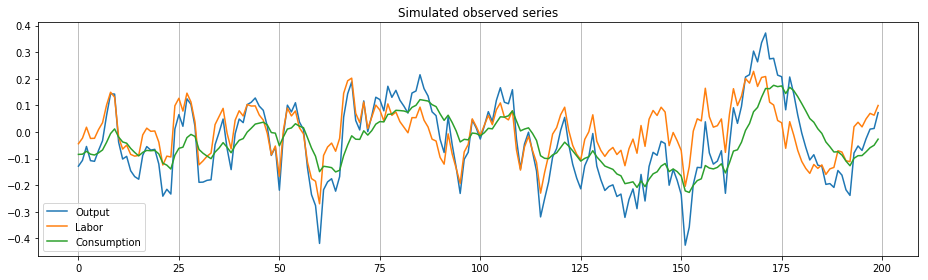
As in Ruge-Murcia (2007), we can simulate the linear model.
np.random.seed(12345)

# Parameters
T = 200   # number of periods to simulate
T0 = 100  # number of initial periods to "burn"

# We can use the exact random draws from "Emsm", downloaded from
# https://sites.google.com/site/frugemurcia/home/replication-files
# on 06/19/2015)
rm2007_eps = [0.0089954547, 0.069601997, -0.0081704445, -0.036704078, -0.026966673, -0.013741121, 0.0089339760, -0.0056557030, -0.0073353523, 0.027214134, 0.0036223219, -0.033331014, 0.032539993, 0.044695276, 0.012599442, -0.020012497, -0.065070833, 0.024777248, -0.058297234, -0.072139533, 0.080062379, 0.023164655, -0.028318809, 0.023734384, -0.023575740, 0.058697373, -0.00080918191, 0.029482310, 0.059178715, -0.010752551, 0.049127695, 0.063137227, -0.015733529, 0.018006224, 0.051256459, -0.014467873, 0.042611930, -0.078176552, -0.0040812905, -0.0086694118, 0.016261678, 0.0055330257, 0.026286130, -0.0066732973, 0.019133914, 0.018442169, 0.0046151171, 0.0015229921, 0.047776839, -0.058401266, 0.014895019, -0.0070732464, -0.036637349, 0.018778403, 0.0030934044, -0.033385312, -0.0044036385, -0.0029289904, -0.029415234, -0.010308393, -0.023496361, -0.023784028, 0.045396730, -0.021532569, -0.086991302, 0.046579589, 0.015086674, 0.0054060766, 0.0094114004, 0.014372645, -0.060998265, -0.0047493261, -0.030991307, -0.022061370, -0.020225482, -0.013470628, -0.013967446, -0.021552474, -0.054801903, -0.0052111107, 0.0080784668, 0.042868645, -0.0015220824, -0.061354829, 0.053529145, -0.020002403, -0.00053686088, 0.085988265, 0.037919020, 0.023531373, 0.0046336046, 0.012880821, 0.0037651140, -0.059647623, -0.027420909, -0.063257854, -0.010324261, -0.025627797, -0.017646345, -0.00091871809, 0.0066086013, 0.0018793222, 0.019543168, -0.031823750, -0.0092249652, 0.013246704, 0.014181125, 0.047271352, 0.047259268, 0.010107337, -0.083925083, -0.036031657, -0.0022387325, -0.035090684, -0.022218572, -0.017554625, 0.033953597, 0.010744674, -0.010891498, -0.0035293110, -0.033522281, -0.072168448, -0.0042416089, -0.025190520, 0.11066349, 0.029308577, -0.018047271, 0.055748729, -0.0016904632, -0.035578602, -0.10830804, -0.013671301, -0.010389470, -0.012295055, 0.055696357, 0.020597878, 0.026447061, -0.054887926, -0.045563156, 0.060229793, 0.028380999, -0.0034341303, 0.038103203, 0.012224323, 0.016752740, -0.0065436404, -0.0010711498, -0.025486203, -0.055621838, 0.0096008728, -0.088779172, 0.092452909, 0.057714587, -0.0057425132, 0.023627700, -0.029821882, -0.012037717, -0.074682148, -0.062682990, -0.038800349, -0.094946077, 0.074545642, -0.00050272713, -0.0075839744, -0.037362343, 0.012332294, 0.10490393, 0.049997520, 0.033916235, -0.061734224, -0.015363425, 0.057711167, -0.051687840, 0.031219589, 0.041031894, 0.0051038726, -0.013144180, 0.054156433, -0.0090438895, 0.023331707, -0.0079434321, -0.0029084658, -0.0064262300, 0.044577448, 0.014816901, 0.043276307, -0.011412684, -0.0026201902, -0.021138420, -0.0020795206, -0.042017897, -0.028148295, 0.063945871, -0.049724502, -0.048571001, -0.061207381, 0.050007129, 0.0062884061, 0.057948665, -0.012780170, -0.020464058, 0.023577863, 0.030007840, -0.013682281, 0.044281158, 0.033864209, -0.016235593, 0.0052712906, 0.035426922, -0.084935662, -0.061241657, 0.038759520, 0.019838792, -0.038971482, -0.043112193, -0.10098203, 0.011744644, 0.014708720, 0.035224935, 0.0098378679, 0.031205446, 0.026015597, -0.048897576, -0.042539822, -0.036330332, -0.033689415, 0.029665808, 0.0086127051, 0.038663112, -0.064534479, -0.036174560, -0.034225451, -0.0084848888, -0.011724560, -0.037544322, -0.013054490, -0.062983798, 0.011448707, 0.0022791918, -0.054508196, 0.046134801, -0.063884585, 0.048918326, 0.018358644, -0.011278321, 0.021175611, -0.0069196463, -0.084987826, 0.016286265, -0.031783692, -0.041129528, -0.11686860, 0.0040626993, 0.057649830, 0.019174675, -0.010319778, 0.080549326, -0.058124228, -0.027757539, -0.0028474062, 0.012399938, -0.088780901, 0.077048657, 0.070548177, -0.023784957, 0.035935388, 0.064960358, 0.019987594, 0.062245578, 0.0014217956, 0.057173164, 0.043800495, -0.023484057, 0.021398628, -0.012723988, 0.012587101, -0.049855702, 0.070557277, -0.017640273, -0.031555592, -0.030900124, -0.028508626, -0.029129143, 0.0024196883, -0.026937200, -0.011642554, -0.045071194, -0.013049519, -0.021908382, 0.017900266, -0.019798107, -0.040774046, -0.027013698, 0.065691125, 0.0081570086, -0.012601818, 0.017918061, 0.017225503, 0.0021227212, 0.032141622, 0]
# Or we can draw our own
gen_eps = np.random.normal(0, reduced_mod1.technology_shock_std, size=(T+T0+1))

eps = rm2007_eps

# Create and solve the model
reduced_mod2 = ReducedRBC2(parameters['value'])
design, transition = reduced_mod2.solve()
selection = np.array([0, 1])

# Generate variables
raw_observed = np.zeros((T+T0+1,3))
raw_state = np.zeros((T+T0+2,2))

for t in range(T+T0+1):
    raw_observed[t] = np.dot(design, raw_state[t])
    raw_state[t+1] = np.dot(transition, raw_state[t]) + selection * eps[t]

# Test that our simulated series are the same as in "Emsm"
# Note: Gauss uses ddof=1 for std dev calculation
assert_allclose(np.mean(raw_state[1:-1,:], axis=0), [-0.0348286036, -0.0133121934])
assert_allclose(np.std(raw_state[1:-1,:], axis=0, ddof=1), [0.122766006, 0.0742206044])
assert_allclose(np.mean(raw_observed[1:,:], axis=0), [-0.027208998, -0.0021226675, -0.025086330])
assert_allclose(np.std(raw_observed[1:,:], axis=0, ddof=1), [0.14527028, 0.089694148, 0.090115364])

# Drop the first 100 observations
sim_observed = raw_observed[T0+1:,:]
sim_state = raw_state[T0+1:-1,:]
fig, ax = plt.subplots(figsize=(13,4))

ax.plot(sim_observed[:,0], label='Output')
ax.plot(sim_observed[:,1], label='Labor')
ax.plot(sim_observed[:,2], label='Consumption')

ax.set_title('Simulated observed series')
ax.xaxis.grid()
ax.legend(loc='lower left')

fig.tight_layout();
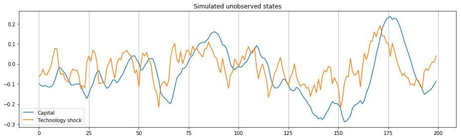
fig, ax = plt.subplots(figsize=(13,4))

ax.plot(sim_state[:,0], label='Capital')
ax.plot(sim_state[:,1], label='Technology shock')

ax.set_title('Simulated unobserved states')
ax.xaxis.grid()
ax.legend(loc='lower left')

fig.tight_layout();
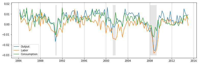
Observed economic data
We use data on hours worked, consumption, and investment
# Get some data
start='1984-01'
end = '2015-01'
labor = DataReader('HOANBS', 'fred', start=start, end=end)        # hours
consumption = DataReader('PCECC96', 'fred', start=start, end=end) # billions of dollars
investment = DataReader('GPDI', 'fred', start=start, end=end)     # billions of dollars
population = DataReader('CNP16OV', 'fred', start=start, end=end)  # thousands of persons
recessions = DataReader('USRECQ', 'fred', start=start, end=end)

# Collect the raw values
raw = pd.concat((labor, consumption, investment, population.resample('QS').mean()), axis=1)
raw.columns = ['labor', 'consumption', 'investment', 'population']
raw['output'] = raw['consumption'] + raw['investment']

# Make the data consistent with the model
y = np.log(raw.output * 10**(9-3) / raw.population)
n = np.log(raw.labor * (1e3 * 40) / raw.population)
c = np.log(raw.consumption * 10**(9-3) / raw.population)

# Make the data stationary
y = y.diff()[1:]
n = n.diff()[1:]
c = c.diff()[1:]

# Construct the final dataset
econ_observed = pd.concat((y, n, c), axis=1)
econ_observed.columns = ['output','labor','consumption']
fig, ax = plt.subplots(figsize=(13,4))

dates = econ_observed.index._mpl_repr()

ax.plot(dates, econ_observed.output, label='Output')
ax.plot(dates, econ_observed.labor, label='Labor')
ax.plot(dates, econ_observed.consumption, label='Consumption')

rec = recessions.resample('QS').last().loc[econ_observed.index[0]:].iloc[:, 0].values
ylim = ax.get_ylim()
ax.fill_between(dates, ylim[0]+1e-5, ylim[1]-1e-5, rec, facecolor='k', alpha=0.1)

ax.xaxis.grid()
ax.legend(loc='lower left');
Estimation
class EstimateRBC1(sm.tsa.statespace.MLEModel):
    def __init__(self, output=None, labor=None, consumption=None,
                 measurement_errors=True,
                 disutility_labor=3, depreciation_rate=0.025,
                 capital_share=0.36, **kwargs):

        # Determine provided observed variables
        self.output = output is not None
        self.labor = labor is not None
        self.consumption = consumption is not None
        self.observed_mask = (
            np.array([self.output, self.labor, self.consumption], dtype=bool)
        )

        observed_variables = np.r_[['output', 'labor', 'consumption']]
        self.observed_variables = observed_variables[self.observed_mask]

        self.measurement_errors = measurement_errors

        # Construct the full endogenous array
        endog = []
        if self.output:
            endog.append(np.array(output))
        if self.labor:
            endog.append(np.array(labor))
        if self.consumption:
            endog.append(np.array(consumption))
        endog = np.c_[endog].transpose()

        # Initialize the statespace model
        super(EstimateRBC1, self).__init__(endog, k_states=2, k_posdef=1, **kwargs)
        self.initialize_stationary()
        self.data.ynames = self.observed_variables

        # Check for stochastic singularity
        if self.k_endog > 1 and not measurement_errors:
            raise ValueError('Stochastic singularity encountered')

        # Save the calibrated parameters
        self.disutility_labor = disutility_labor
        self.depreciation_rate = depreciation_rate
        self.capital_share = capital_share

        # Create the structural model
        self.structural = ReducedRBC2()

        # Setup fixed elements of the statespace matrices
        self['selection', 1, 0] = 1

        idx = np.diag_indices(self.k_endog)
        self._idx_obs_cov = ('obs_cov', idx[0], idx[1])

    @property
    def start_params(self):
        start_params = [0.99, 0.5, 0.01]
        if self.measurement_errors:
            start_meas_error = np.r_[[0.1]*3]
            start_params += start_meas_error[self.observed_mask].tolist()

        return start_params

    @property
    def param_names(self):
        param_names = ['beta', 'rho', 'sigma.vareps']
        if self.measurement_errors:
            meas_error_names = np.r_[['sigma2.y', 'sigma2.n', 'sigma2.c']]
            param_names += meas_error_names[self.observed_mask].tolist()

        return param_names

    def transform_params(self, unconstrained):
        constrained = np.zeros(unconstrained.shape, unconstrained.dtype)

        # Discount rate is between 0 and 1
        constrained[0] = max(1 / (1 + np.exp(unconstrained[0])) - 1e-4, 1e-4)
        # Technology shock persistence is between -1 and 1
        constrained[1] = unconstrained[1] / (1 + np.abs(unconstrained[1]))
        # Technology shock std. dev. is positive
        constrained[2] = np.abs(unconstrained[2])
        # Measurement error variances must be positive
        if self.measurement_errors:
            constrained[3:3+self.k_endog] = unconstrained[3:3+self.k_endog]**2

        return constrained

    def untransform_params(self, constrained):
        unconstrained = np.zeros(constrained.shape, constrained.dtype)

        # Discount rate is between 0 and 1
        unconstrained[0] = np.log((1 - constrained[0] + 1e-4) / (constrained[0] + 1e-4))
        # Technology shock persistence is between -1 and 1
        unconstrained[1] = constrained[1] / (1 + constrained[1])
        # Technology shock std. dev. is positive
        unconstrained[2] = constrained[2]
        # Measurement error variances must be positive
        if self.measurement_errors:
            unconstrained[3:3+self.k_endog] = constrained[3:3+self.k_endog]**0.5

        return unconstrained

    def update(self, params, **kwargs):
        params = super(EstimateRBC1, self).update(params, **kwargs)

        # Get the parameters of the structural model
        # Note: we are calibrating three parameters
        structural_params = np.r_[
            params[0],
            self.disutility_labor,
            self.depreciation_rate,
            self.capital_share,
            params[1:3]
        ]

        # Solve the model
        design, transition = self.structural.solve(structural_params)

        # Update the statespace representation
        self['design'] = design[self.observed_mask, :]
        if self.measurement_errors:
            self[self._idx_obs_cov] = params[3:3+self.k_endog]
        self['transition'] = transition
        self['state_cov', 0, 0] = self.structural.technology_shock_std**2
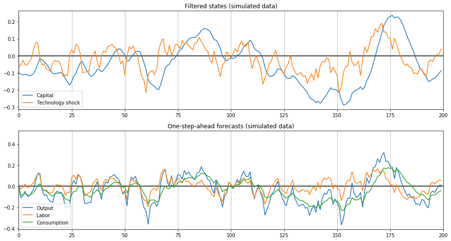
Estimation on simulated data
# Setup the statespace model
sim_mod = EstimateRBC1(
    output=sim_observed[:,0],
    labor=sim_observed[:,1],
    consumption=sim_observed[:,2],
    measurement_errors=True
)

# sim_res = sim_mod.fit(maxiter=1000, information_matrix_type='oim')
sim_res = sim_mod.fit(maxiter=1000)

print(sim_res.summary())
/Users/fulton/miniconda3/envs/python3/lib/python3.6/site-packages/ipykernel_launcher.py:75: RuntimeWarning: overflow encountered in exp


                                  Statespace Model Results
============================================================================================
Dep. Variable:     ['output' 'labor' 'consumption']   No. Observations:                  200
Model:                                 EstimateRBC1   Log Likelihood                3160.668
Date:                              Thu, 01 Nov 2018   AIC                          -6309.336
Time:                                      20:36:40   BIC                          -6289.546
Sample:                                           0   HQIC                         -6301.328
                                              - 200
Covariance Type:                                opg
================================================================================
                   coef    std err          z      P>|z|      [0.025      0.975]
--------------------------------------------------------------------------------
beta             0.9500   5.57e-06    1.7e+05      0.000       0.950       0.950
rho              0.8499    8.3e-05   1.02e+04      0.000       0.850       0.850
sigma.vareps     0.0440   1.23e-06   3.58e+04      0.000       0.044       0.044
sigma2.y      5.362e-10   5.39e-09      0.099      0.921      -1e-08    1.11e-08
sigma2.n      4.172e-05   8.27e-05      0.504      0.614      -0.000       0.000
sigma2.c       8.71e-13   4.81e-09      0.000      1.000   -9.43e-09    9.43e-09
======================================================================================
Ljung-Box (Q):          40.66, 0.21, 79.19   Jarque-Bera (JB):   0.09, 318540.26, 0.08
Prob(Q):                  0.44, 1.00, 0.00   Prob(JB):                0.95, 0.00, 0.96
Heteroskedasticity (H):   0.86, 0.00, 0.66   Skew:                  -0.05, 13.96, 0.04
Prob(H) (two-sided):      0.54, 0.00, 0.09   Kurtosis:              2.95, 196.51, 2.93
======================================================================================

Warnings:
[1] Covariance matrix calculated using the outer product of gradients (complex-step).
[2] Covariance matrix is singular or near-singular, with condition number 5.64e+18. Standard errors may be unstable.


/Users/fulton/projects/statsmodels/statsmodels/base/model.py:508: ConvergenceWarning: Maximum Likelihood optimization failed to converge. Check mle_retvals
  "Check mle_retvals", ConvergenceWarning)
fig, axes = plt.subplots(2, 1, figsize=(13,7))

# Filtered states confidence intervals
states_cov = np.diagonal(sim_res.filtered_state_cov).T
states_upper = sim_res.filtered_state + 1.96 * states_cov**0.5
states_lower = sim_res.filtered_state - 1.96 * states_cov**0.5

ax = axes[0]
lines, = ax.plot(sim_res.filtered_state[0], label='Capital')
ax.fill_between(states_lower[0], states_upper[0], color=lines.get_color(), alpha=0.2)

lines, = ax.plot(sim_res.filtered_state[1], label='Technology shock')
ax.fill_between(states_lower[1], states_upper[1], color=lines.get_color(), alpha=0.2)

ax.set_xlim((0, 200))
ax.hlines(0, 0, 200)

ax.set_title('Filtered states (simulated data)')
ax.legend(loc='lower left')
ax.xaxis.grid()

ax = axes[1]

# One-step-ahead forecasts confidence intervals
forecasts_cov = np.diagonal(sim_res.forecasts_error_cov).T
forecasts_upper = sim_res.forecasts + 1.96 * forecasts_cov**0.5
forecasts_lower = sim_res.forecasts - 1.96 * forecasts_cov**0.5

for i in range(sim_mod.k_endog):
    lines, = ax.plot(sim_res.forecasts[i], label=sim_mod.endog_names[i].title())
    ax.fill_between(forecasts_lower[i], forecasts_upper[i], color=lines.get_color(), alpha=0.1)

ax.set_xlim((0, 200))
ax.hlines(0, 0, 200)

ax.set_title('One-step-ahead forecasts (simulated data)')
ax.legend(loc='lower left')
ax.xaxis.grid()

fig.tight_layout();
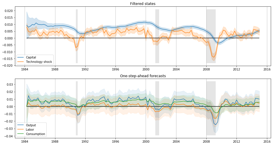
Estimation on observed data
# Setup the statespace model
econ_mod = EstimateRBC1(
    output=econ_observed['output'],
    labor=econ_observed['labor'],
    consumption=econ_observed['consumption'],
    measurement_errors=True,
    dates=econ_observed.index
)

econ_res = econ_mod.fit(maxiter=1000, information_matrix_type='oim')

print(econ_res.summary())
                                  Statespace Model Results
============================================================================================
Dep. Variable:     ['output' 'labor' 'consumption']   No. Observations:                  124
Model:                                 EstimateRBC1   Log Likelihood                1446.774
Date:                              Thu, 01 Nov 2018   AIC                          -2881.547
Time:                                      20:36:43   BIC                          -2864.625
Sample:                                  04-01-1984   HQIC                         -2874.673
                                       - 01-01-2015
Covariance Type:                                opg
================================================================================
                   coef    std err          z      P>|z|      [0.025      0.975]
--------------------------------------------------------------------------------
beta             0.9850      0.010     96.667      0.000       0.965       1.005
rho              0.9616      0.023     42.722      0.000       0.918       1.006
sigma.vareps     0.0022      0.000      9.797      0.000       0.002       0.003
sigma2.y       9.75e-06   2.58e-06      3.775      0.000    4.69e-06    1.48e-05
sigma2.n      2.398e-05   4.66e-06      5.143      0.000    1.48e-05    3.31e-05
sigma2.c      1.568e-05   2.16e-06      7.251      0.000    1.14e-05    1.99e-05
=====================================================================================
Ljung-Box (Q):          38.83, 120.95, 47.83   Jarque-Bera (JB):    16.90, 0.23, 3.25
Prob(Q):                    0.52, 0.00, 0.18   Prob(JB):             0.00, 0.89, 0.20
Heteroskedasticity (H):     1.68, 0.90, 0.53   Skew:                0.40, -0.11, 0.32
Prob(H) (two-sided):        0.10, 0.74, 0.05   Kurtosis:             4.62, 3.01, 3.46
=====================================================================================

Warnings:
[1] Covariance matrix calculated using the outer product of gradients (complex-step).
fig, axes = plt.subplots(2, 1, figsize=(13,7))

# Filtered states confidence intervals
states_cov = np.diagonal(econ_res.filtered_state_cov).T
states_upper = econ_res.filtered_state + 1.96 * states_cov**0.5
states_lower = econ_res.filtered_state - 1.96 * states_cov**0.5

ax = axes[0]
lines, = ax.plot(dates, econ_res.filtered_state[0], label='Capital')
ax.fill_between(dates, states_lower[0], states_upper[0], color=lines.get_color(), alpha=0.2)

lines, = ax.plot(dates, econ_res.filtered_state[1], label='Technology shock')
ax.fill_between(dates, states_lower[1], states_upper[1], color=lines.get_color(), alpha=0.2)

ylim = ax.get_ylim()
ax.fill_between(dates, ylim[0]+1e-4, ylim[1]-1e-4, rec, facecolor='k', alpha=0.1)

ax.hlines(0, dates[0], dates[-1])

ax.set_title('Filtered states')
ax.legend(loc='lower left')
ax.xaxis.grid()

ax = axes[1]

# One-step-ahead forecasts confidence intervals
forecasts_cov = np.diagonal(econ_res.forecasts_error_cov).T
forecasts_upper = econ_res.forecasts + 1.96 * forecasts_cov**0.5
forecasts_lower = econ_res.forecasts - 1.96 * forecasts_cov**0.5

for i in range(econ_mod.k_endog):
    lines, = ax.plot(dates, econ_res.forecasts[i], label=econ_mod.endog_names[i].title())
    ax.fill_between(dates, forecasts_lower[i], forecasts_upper[i], color=lines.get_color(), alpha=0.1)

ylim = ax.get_ylim()
ax.fill_between(dates, ylim[0]+1e-4, ylim[1]-1e-4, rec, facecolor='k', alpha=0.1)

ax.hlines(0, dates[0], dates[-1])

ax.set_title('One-step-ahead forecasts')
ax.legend(loc='lower left')
ax.xaxis.grid()

fig.tight_layout();
References
[1] DeJong, David N., and Chetan Dave. 2011.
    Structural Macroeconometrics. Second edition.
    Princeton: Princeton University Press.
[2] Ruge-Murcia, Francisco J. 2007.
    "Methods to Estimate Dynamic Stochastic General Equilibrium Models."
    Journal of Economic Dynamics and Control 31 (8): 2599–2636.